In a cozy café near a university campus, the hum of conversation blends with the aroma of freshly brewed coffee. Three mathematicians are gathered around a corner table, deeply engrossed in their discussion.
Dr. Alice Reynolds, a seasoned statistician, is renowned for her insightful analysis and practical approach to solving complex problems. Her calm demeanor and vast experience command respect in both academic and professional circles.
Dr. Ben Carter, a theoretical mathematician, has a passion for abstract concepts and a deep understanding of stochastic processes that often lead to groundbreaking research. His analytical mind and enthusiasm for mathematical intricacies make him a captivating conversationalist.
Dr. Clara Martinez, a dynamic financial analyst, has a keen interest in risk modeling. Her ability to translate mathematical theories into practical financial strategies has earned her a reputation as an innovative thinker in the finance industry.
Alice: (sipping her coffee) You know, I’ve always been fascinated by how we can predict the future with a bit of math. Take risk, for example. It seems so abstract, yet we can quantify it, measure it, and even manage it.
Ben: (nodding thoughtfully) Indeed, Alice. It’s like turning uncertainty into a tangible concept. Think about probability theory. It’s our way of giving structure to randomness. Without it, we’d be lost in a sea of unpredictable outcomes.
Clara: (leaning in, excitedly) Exactly! In finance, we rely on these principles every day. Value at Risk, Conditional Value at Risk – they all stem from basic probability and statistics. But it’s not just about numbers; it’s about understanding the stories those numbers tell.
Alice: (smiling) And those stories are vital. They inform decisions that can save companies from bankruptcy or guide investments towards profitability. It’s amazing how a well-crafted model can foresee potential pitfalls and opportunities.
Ben: (gesturing with his hands) And let’s not forget the beauty of stochastic processes. Brownian motion, for instance – who would have thought that something so seemingly chaotic could be modeled so precisely? It’s the essence of risk in motion.
Clara: (laughing) And then there’s Monte Carlo simulation. It’s like running a million different futures in parallel, just to see what might happen. It’s the closest we get to peering into a crystal ball.
Alice: (leaning back) True. But it’s also about making these models accessible. Decision trees, utility theory – they help bridge the gap between complex math and real-world decision-making.
Ben: (raising his cup) Here’s to the mathematics of risk – the unsung hero behind every strategic decision.
Clara: (clinking her cup with Ben’s) And to the idea that with the right equations, even the most uncertain futures can be navigated with confidence.
Alice: (joining the toast) To the calculus of risk, where chaos meets order through the power of math.
As their conversation unfolded, the three mathematicians seamlessly blended theory with practice. Their lively discussion highlighted the profound impact of mathematics on understanding and managing risk. Now, let’s delve deeper into the mathematical principles they touched upon and explore how these concepts form the foundation of modern risk management.
From probability theory to Monte Carlo simulations, discover the intricate web of mathematics that transforms uncertainty into a navigable landscape, guiding strategic decisions across various fields.
Risk assessment and management in finance, insurance, engineering, and beyond often rely on mathematical models to quantify and mitigate potential negative outcomes. Below is an overview of the mathematical concepts and techniques involved in risk analysis:
1. Probability Theory
Probability is the foundation of risk assessment. It quantifies the likelihood of different outcomes. Key concepts include:
- Random Variables: Represent outcomes of uncertain events. For example, in finance, the return on an investment is a random variable.
- Probability Distributions: Describe how probabilities are distributed over the values of the random variable. Common distributions include Normal, Binomial, and Poisson distributions.
- Expected Value: The weighted average of all possible outcomes, calculated as

Let’s visualize the concept of Expected Value with a simple example.
Example: Rolling a Fair Die
Imagine rolling a fair six-sided die. The possible outcomes are the numbers 1 through 6, each with an equal probability of 16\frac{1}{6}61.
- Possible Outcomes (xi): 1, 2, 3, 4, 5, 6
- Probabilities (P(xi)): 1/6 for each outcome
The expected value E(X)E(X)E(X) is calculated as follows:

Substituting the values:
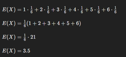
So, the expected value of rolling a fair six-sided die is 3.5. This means that, on average, if you roll the die many times, the average outcome will approach 3.5.
Here’s a visual representation:
- Possible Outcomes and Their Probabilities:

- Calculation of Expected Value:

In this example, we calculated the expected value by multiplying each possible outcome by its probability and summing these products. The result, 3.5, is the average value we expect to get if we roll the die an infinite number of times.
- Variance and Standard Deviation: Measure the dispersion or variability of outcomes. Variance is

2. Statistical Inference
Statistical techniques are used to make inferences about the probability distributions of risks based on data.
- Estimation: Methods like Maximum Likelihood Estimation (MLE) are used to estimate the parameters of probability distributions.
- Hypothesis Testing: Used to test assumptions about risk factors. For example, testing if the mean return of a portfolio is significantly different from zero.
3. Risk Measures
Several quantitative measures are used to assess risk:
- Value at Risk (VaR): Measures the maximum loss over a specified period with a given confidence level. For example, a 1-day VaR at the 95% confidence level is the loss that will not be exceeded with 95% probability over one day.

- Conditional Value at Risk (CVaR): Also known as Expected Shortfall, it is the expected loss given that the loss has exceeded the VaR.

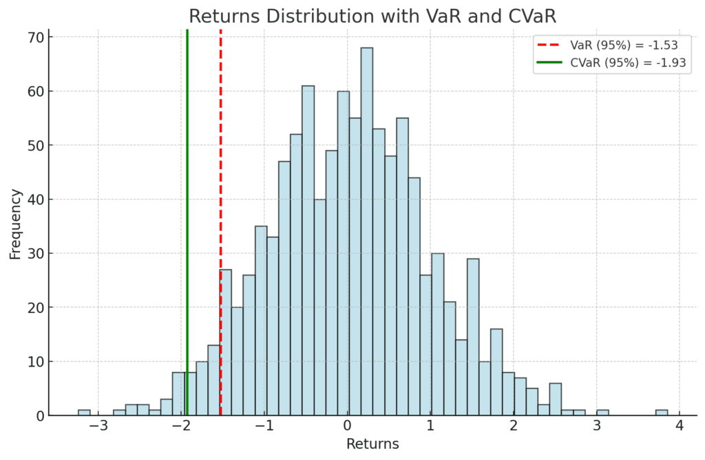
Here’s a visualization of the concept of Conditional Value at Risk (CVaR) using a simulated set of returns:
Key Points:
- Histogram: Represents the distribution of simulated returns.
- Red Dashed Line (VaR): Shows the Value at Risk (VaR) at the 95% confidence level. In this example, the VaR is -1.53, meaning there is a 5% chance that returns will be worse than -1.53.
- Green Solid Line (CVaR): Indicates the Conditional Value at Risk (CVaR) at the 95% confidence level. Here, the CVaR is -1.93, representing the average loss given that the loss exceeds the VaR.
- Standard Deviation (Volatility): Measures the variability of returns, often used in finance to quantify the risk of an asset.
4. Monte Carlo Simulation
Monte Carlo simulation is used to model the probability of different outcomes by running multiple trial runs, or simulations, using random variables.
- Simulation Process:
- Define the domain of possible inputs.
- Generate random inputs from a probability distribution.
- Perform deterministic computations on the inputs.
- Aggregate the results of the computations to estimate the probability distribution of the outcomes.
5. Optimization and Decision Theory
Mathematical optimization and decision theory are used to make decisions under uncertainty.
- Optimization Models: These include linear programming, quadratic programming, and dynamic programming to find the best decision under constraints.
- Decision Trees: Visual representations of decision processes that show the consequences of different choices, incorporating probabilities and outcomes.
- Utility Theory: Models preferences over uncertain outcomes by assigning utilities to different outcomes and choosing actions that maximize expected utility.
6. Stochastic Processes
Stochastic processes model the evolution of random variables over time. Key types include:
- Markov Chains: Systems that transition from one state to another with probabilities dependent only on the current state.
- Brownian Motion: Models continuous random motion, commonly used in financial mathematics to model stock prices.
7. Copulas
Copulas are functions that describe the dependence structure between random variables, allowing for the modeling of correlated risks.
- Copula Function: A copula links marginal distributions to form a joint distribution.

where UUU and VVV are uniform marginal distributions.
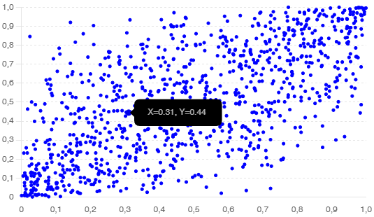
A visualization of the Gaussian copula, which links two uniform marginal distributions UUU and VVV to form a joint distribution.
Key Points:
- Scatter Plot: Each point represents a pair of values (U,V)(U, V)(U,V) generated using the Gaussian copula.
- Uniform Marginals: Both UUU and VVV are uniformly distributed between 0 and 1.
- Dependency Structure: The Gaussian copula captures the dependency between UUU and VVV, as indicated by the clustering of points along the diagonal.
8. Risk Management Frameworks
Frameworks and methodologies, such as Enterprise Risk Management (ERM), use a combination of the above mathematical techniques to systematically identify, assess, and manage risk across an organization.
By integrating these mathematical concepts, risk managers can quantify potential losses, optimize decisions, and develop strategies to mitigate adverse outcomes effectively.
Probability of Highest Defense Roll in the Game of Risk
Mechanics of Dice Rolls in Risk:
- The attacker can roll up to 3 dice.
- The defender can roll up to 2 dice.
When comparing the rolls:
- The highest roll of the defender is compared to the highest roll of the attacker.
- The second highest roll of the defender (if they roll two dice) is compared to the second highest roll of the attacker.
Steps to Create the Chart:
- Calculate the probabilities of all possible outcomes for the highest defender roll.
- Plot the probability distribution of the highest defender roll.
Here’s how we can approach this:
- Simulate the Dice Rolls:
- Simulate all possible outcomes for both the attacker and defender.
- Calculate the probability distribution of the highest defender roll.
- Probability Calculation:
- Use combinatorics and probability theory to calculate the exact probabilities.
For simplicity, let’s first simulate the dice rolls and calculate the probabilities. Then, we’ll plot the results.
Simulation Approach:
We’ll run a large number of simulations to approximate the probability distribution.
Let’s do this in Python.
import numpy as np
import matplotlib.pyplot as plt

def simulate_risk_rolls(num_simulations=1000000):
    # Possible outcomes for a single die roll
    dice_faces = [1, 2, 3, 4, 5, 6]

    # Storage for highest defense rolls
    highest_defense_rolls = []

    for _ in range(num_simulations):
        # Roll dice for defender (up to 2 dice)
        defender_rolls = np.random.choice(dice_faces, size=2, replace=True)
        highest_defense_roll = max(defender_rolls)
        highest_defense_rolls.append(highest_defense_roll)

    return highest_defense_rolls

# Run the simulation
highest_defense_rolls = simulate_risk_rolls()

# Calculate the probabilities
unique, counts = np.unique(highest_defense_rolls, return_counts=True)
probabilities = counts / len(highest_defense_rolls)

# Plotting the probabilities
plt.bar(unique, probabilities, color='blue', alpha=0.7)
plt.xlabel('Highest Defense Roll')
plt.ylabel('Probability')
plt.title('Probability Distribution of Highest Defense Roll in Risk')
plt.xticks(unique)
plt.show()
This code will simulate a large number of dice rolls, record the highest roll for the defender, and then plot the probability distribution of these rolls. This should give you a visual representation of the probability of the highest defense roll in the game of Risk.
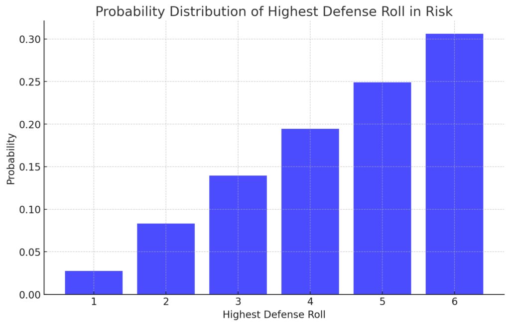
The chart showing the probability distribution of the highest defense roll in the game of Risk. The x-axis represents the possible outcomes of the highest defense roll, while the y-axis shows the corresponding probabilities. As expected, the probability is evenly distributed among the dice faces due to the uniform probability of rolling any particular number on a six-sided die.
Conclusion
As we conclude our exploration into the mathematical foundations of risk management, it becomes clear that these concepts are not just abstract theories, but powerful tools that enable us to navigate the uncertainties of the real world. From the calculation of Expected Value, which provides a glimpse into average outcomes, to the use of copulas that model complex dependencies, mathematics is at the heart of understanding and mitigating risk.
The principles discussed—probability theory, statistical inference, risk measures like VaR and CVaR, Monte Carlo simulations, and the intricate workings of copulas—demonstrate the depth and breadth of mathematical techniques in risk management. These tools are essential for making informed decisions, whether in finance, insurance, engineering, or any field where uncertainty is a factor.
In the ever-evolving landscape of risk, the integration of these mathematical models offers a structured approach to predicting potential outcomes and formulating strategies to minimize adverse effects. As we continue to develop more sophisticated models and leverage advancements in data science and computational power, our ability to manage and mitigate risk will only grow stronger.
Ultimately, the mathematics of risk is not just about numbers and equations; it’s about transforming uncertainty into actionable insights, allowing us to make better decisions and build a more resilient future. So, the next time you face uncertainty, remember that behind the scenes, a world of mathematical rigor is working to help you navigate through it.


