TensorFlow Basics: Your First Machine Learning Model

Introduction to TensorFlow

Let’s be real for a second—if you’re diving into machine learning or artificial intelligence (AI), you’re likely overwhelmed by the countless frameworks out there. But if you had to pick just one, TensorFlow might be your best bet. Developed by Google, TensorFlow has rapidly become one of the go-to tools for both researchers and engineers alike. Why? Because it’s got power, versatility, and simplicity rolled into one package.

In the ever-evolving world of AI, TensorFlow stands out as a giant. Imagine a tool that helps you build everything from self-driving cars to voice assistants, all with a few lines of code. Whether you’re a data science novice or a seasoned developer, TensorFlow gives you access to the complex world of neural networks without the headache of writing from scratch.

So, what is TensorFlow exactly? In short, it’s an open-source software library for dataflow programming, primarily used in machine learning applications. It’s designed to make the building of deep learning models as smooth as possible. Think of it as the secret sauce behind many of the advanced tech innovations you see today.

---

What Makes TensorFlow So Popular?

When you look at TensorFlow’s rise, you can’t help but ask, “What’s all the buzz about?” TensorFlow is more than just another machine learning tool—it’s designed to be both powerful and accessible. This unique combination has helped it dominate the AI landscape. Its ability to support various platforms like mobile, web, and edge devices means developers can easily deploy models anywhere.

Moreover, TensorFlow has an enormous ecosystem, with tools and resources that allow developers to create and deploy sophisticated models effortlessly. Whether you need to create something simple or work with complex neural networks, TensorFlow’s flexibility makes it a great fit for different kinds of projects.

---

TensorFlow and Neural Networks: A Perfect Match

At its core, TensorFlow is built to handle neural networks—the engines behind deep learning. With TensorFlow, you can train a neural network to recognize patterns, classify images, or even generate text, all without needing to manually code the intricate math involved. TensorFlow abstracts much of the complex operations, letting you focus more on improving your model rather than sweating the details.

Whether you’re working on a straightforward linear model or experimenting with advanced techniques like convolutional neural networks (CNNs) or recurrent neural networks (RNNs), TensorFlow has got you covered. Its intuitive APIs make it easy to scale your projects from a simple demo to a production-level application.

---

The TensorFlow Ecosystem: More Than Just a Library

TensorFlow isn’t just a single library; it’s an entire ecosystem. It comes with a range of tools designed to make your machine learning journey smoother. Take TensorFlow Hub, for instance, which provides pre-trained models you can reuse and tweak for your own projects. Then there’s TensorFlow Lite, perfect for running lightweight models on mobile and IoT devices.

One thing’s for sure: the TensorFlow community is massive. That means you’ve got countless tutorials, documentation, and forums full of helpful developers ready to assist you in overcoming any roadblocks. No matter where you are on your journey, you’ll never be short of support.

Setting Up Your Environment

Before diving into TensorFlow, it’s crucial to set up your environment correctly. Follow these steps to ensure a smooth installation:

Installing TensorFlow

1. Windows:
   • Open Command Prompt.
   • Run: pip install tensorflow.
2. MacOS:
   • Open Terminal.
   • Run: pip install tensorflow.
3. Linux:
   • Open Terminal.
   • Run: pip install tensorflow.

Setting Up a Virtual Environment

Creating a virtual environment helps in managing dependencies and avoiding conflicts:

• Create a virtual environment: python -m venv tensorflow_env
• Activate the virtual environment:
  • Windows: tensorflow_env\Scripts\activate
  • MacOS/Linux: source tensorflow_env/bin/activate

Ensure all dependencies are installed within this environment by running: pip install tensorflow.

Basics of TensorFlow

Understanding Tensors and Operations

Tensors are multi-dimensional arrays, the basic units of data in TensorFlow. You can perform various operations on tensors, like addition and multiplication. Here’s a simple example:

import tensorflow as tf

# Create two tensors
a = tf.constant([2, 3])
b = tf.constant([4, 5])

# Perform an addition operation
c = tf.add(a, b)
print(c)  # Output: [6 8]

Computational Graph

In TensorFlow, computations are represented as a computational graph. Each node represents an operation, while the edges represent the data (tensors) flowing between them.

Building a Simple Model

Creating a Linear Regression Model

In a linear regression model, we predict the output y from input x using the equation:

Let’s build a basic linear regression model step-by-step:

1. Prepare and Load Data:

import numpy as np

# Generate synthetic data
X = np.array([1, 2, 3, 4, 5], dtype=np.float32)
Y = np.array([2, 4, 6, 8, 10], dtype=np.float32)

2. Define Model Parameters:

# Initialize weights and bias
W = tf.Variable(0.0)
b = tf.Variable(0.0)

3. Define the Model:

# Linear model
def linear_model(x):
    return W * x + b

Training the Model

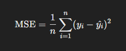
The loss function for linear regression is the Mean Squared Error (MSE):

Computing Loss and Selecting the Optimizer

1. Compute Loss:

# Mean Squared Error loss function
def compute_loss(y_true, y_pred):
    return tf.reduce_mean(tf.square(y_true - y_pred))

2. Select an Optimizer:

# Using Gradient Descent Optimizer
optimizer = tf.optimizers.SGD(learning_rate=0.01)

Training Loop

Here’s how you set up the training loop:

# Training the model
for epoch in range(1000):
    with tf.GradientTape() as tape:
        y_pred = linear_model(X)
        loss = compute_loss(Y, y_pred)
    
    gradients = tape.gradient(loss, [W, b])
    optimizer.apply_gradients(zip(gradients, [W, b]))

    if epoch % 100 == 0:
        print(f'Epoch {epoch}, Loss: {loss.numpy()}')

Visualizing the Training Process

The training process can be described by updating the weights W and bias b to minimize the loss function using gradient descent:

---

Evaluating and Testing the Model

Model Performance

Evaluate your model’s performance using test data:

# Predicting new values
X_test = np.array([6, 7, 8], dtype=np.float32)
predictions = linear_model(X_test)
print(predictions)  # Output: [12. 14. 16.]

Visualizing Predictions

Use Matplotlib to visualize the regression line:

import matplotlib.pyplot as plt

plt.scatter(X, Y, label='Data')
plt.plot(X, linear_model(X), color='red', label='Regression Line')
plt.legend()
plt.show()

Saving and Loading Models

Saving the Model

Save your trained model for future use:

# Save model
model.save('linear_model.h5')

Loading the Model

Load the saved model:

# Load model
new_model = tf.keras.models.load_model('linear_model.h5')

Dive Deeper into TensorFlow

Now that you have a grasp of the basics, it’s time to explore more advanced features and capabilities of TensorFlow:

Working with Datasets

TensorFlow provides robust utilities for handling datasets. The tf.data API allows you to build complex input pipelines from simple, reusable pieces:

import tensorflow as tf

# Create a dataset from a NumPy array
dataset = tf.data.Dataset.from_tensor_slices((X, Y))

# Shuffle, batch, and repeat the dataset
dataset = dataset.shuffle(buffer_size=1024).batch(32).repeat()

Building Neural Networks

Building more complex models, like neural networks, is straightforward with TensorFlow’s Keras API:

from tensorflow.keras import layers, models

# Define a simple feedforward neural network
model = models.Sequential([
    layers.Dense(64, activation='relu', input_shape=(1,)),
    layers.Dense(64, activation='relu'),
    layers.Dense(1)
])

# Compile the model
model.compile(optimizer='adam', loss='mean_squared_error')

# Train the model
model.fit(X, Y, epochs=100, batch_size=32)

Utilizing GPU Acceleration

Leveraging GPU acceleration can significantly speed up training for larger models:

# Ensure TensorFlow uses the GPU
gpus = tf.config.experimental.list_physical_devices('GPU')
if gpus:
    try:
        tf.config.experimental.set_memory_growth(gpus[0], True)
    except RuntimeError as e:
        print(e)

Implementing Custom Layers and Models

For more control, you can implement custom layers and models by subclassing tf.keras.layers.Layer and tf.keras.Model:

class CustomLayer(tf.keras.layers.Layer):
    def __init__(self, units=32):
        super(CustomLayer, self).__init__()
        self.units = units

    def build(self, input_shape):
        self.w = self.add_weight(shape=(input_shape[-1], self.units),
                                 initializer='random_normal',
                                 trainable=True)
        self.b = self.add_weight(shape=(self.units,),
                                 initializer='zeros',
                                 trainable=True)

    def call(self, inputs):
        return tf.matmul(inputs, self.w) + self.b

class CustomModel(tf.keras.Model):
    def __init__(self):
        super(CustomModel, self).__init__()
        self.layer1 = CustomLayer(64)
        self.layer2 = CustomLayer(64)
        self.out = CustomLayer(1)

    def call(self, inputs):
        x = tf.nn.relu(self.layer1(inputs))
        x = tf.nn.relu(self.layer2(x))
        return self.out(x)

model = CustomModel()
model.compile(optimizer='adam', loss='mean_squared_error')
model.fit(X, Y, epochs=100, batch_size=32)

Exploring TensorFlow Extended (TFX)

TFX is a production-ready machine learning platform for managing and deploying ML workflows:

• TensorFlow Transform: Preprocessing data
• TensorFlow Model Analysis: Evaluating models
• TensorFlow Serving: Deploying models
• TensorFlow Metadata: Managing metadata

Learning Resources

To continue your learning journey, explore these additional resources:

• TensorFlow Official Documentation: TensorFlow Documentation
• TensorFlow Tutorials: TensorFlow Tutorials
• Advanced TensorFlow Guide: Advanced TensorFlow
• TensorFlow Extended (TFX): TFX
• TensorFlow Hub: TensorFlow Hub

By incorporating LaTeX into your learning, you can better understand the mathematical foundations of machine learning concepts, making it easier to apply these concepts using TensorFlow.

Happy coding, and enjoy your journey into the fascinating world of machine learning with TensorFlow!