
What Are t-SNE and UMAP? A Quick Overview
When dealing with complex, high-dimensional data, trying to make sense of it visually can feel like walking through fog.
Dimensionality reduction techniques like t-SNE and UMAP clear up that fog, helping us understand and visualize intricate patterns.
But what exactly are they?
t-SNE (t-distributed Stochastic Neighbor Embedding) and UMAP (Uniform Manifold Approximation and Projection) are two popular algorithms used for this purpose. Both excel at simplifying multi-dimensional data into 2D or 3D for easy interpretation. While they may seem similar on the surface, their underlying mechanics and the types of insights they provide can be surprisingly different.
Both tools are ideal when you need a snapshot of how data points cluster, but choosing one over the other depends heavily on the dataset and the goals of your analysis.
The Purpose of Dimensionality Reduction Explained
Before diving into the details of t-SNE and UMAP, let’s take a step back. What is dimensionality reduction, and why is it so crucial? In the simplest terms, it’s about taking data with a high number of features or dimensions (think spreadsheets with hundreds of columns) and reducing them to just a few. But, there’s a trick: you still need to maintain the essence of the data.
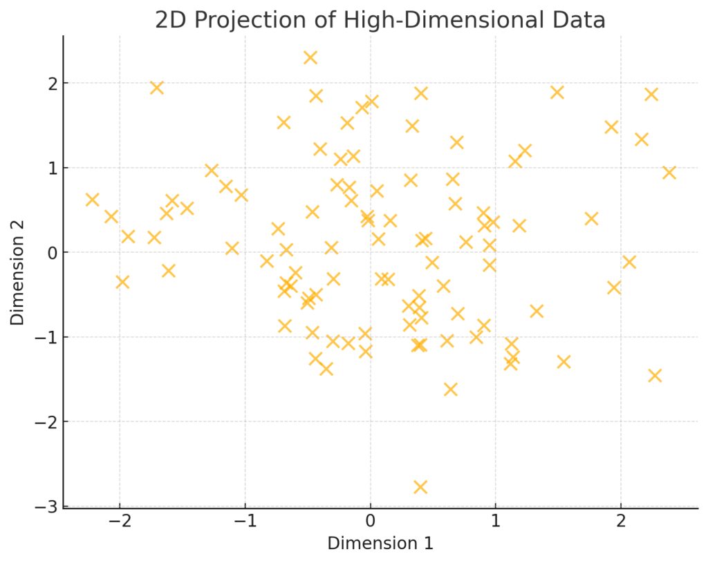
In real-world datasets, many dimensions don’t contribute meaningful differences between data points. Dimensionality reduction helps you filter out the noise, letting you see relationships and clusters that might otherwise go unnoticed.
For instance, when working with gene expression data or image embeddings, the real magic happens when complex patterns are condensed into a visual format. t-SNE and UMAP both achieve this, but they do it differently. Let’s unpack how.
How t-SNE Works: Pros and Cons
t-SNE operates by transforming high-dimensional distances into probabilities. In simple terms, it tries to keep points that were close in high-dimensional space still close when projected into 2D or 3D. At its core, t-SNE is great at capturing local relationships—how nearby points interact and cluster.
However, it comes with some baggage. One of the most well-known drawbacks is computational cost. t-SNE can be slow, especially on larger datasets. Plus, the algorithm’s focus on local structure can cause the global arrangement of clusters to get lost, making it harder to understand the big picture of your data.
That said, for smaller datasets or cases where local relationships are key, t-SNE is a powerful choice.
UMAP: A Faster, More Flexible Alternative?
While t-SNE has earned its place, UMAP emerged to address some of its weaknesses, particularly around speed and flexibility. UMAP takes a different mathematical approach based on topology. Without diving into the weeds, this means UMAP attempts to preserve both local and global structure, giving you a better sense of the full data landscape.
Speed is one of UMAP’s major selling points. On large datasets, UMAP often runs significantly faster than t-SNE, and in some cases, it can handle millions of points with relative ease. UMAP also offers more control through hyperparameters, allowing for finer customization depending on your data needs.
If you’re dealing with vast datasets and need a quick snapshot without sacrificing quality, UMAP is often the go-to.
Visualizing Data: t-SNE vs UMAP
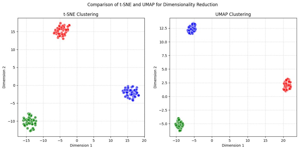
When you see the results of t-SNE and UMAP side by side, the differences in visualization can be striking. t-SNE tends to show tighter, more compact clusters, with clear separations between local groups. It’s excellent for finding small clusters or groups that are tightly related. This makes it ideal for single-cell RNA-seq data or small biological datasets where tight clustering is essential.
On the other hand, UMAP’s plots often look more spread out, but they provide a more holistic picture. The clusters might not be as tight, but the global structure—the relationship between distant points—tends to be clearer. This can be important when you’re trying to see how various groups in your data relate to each other, especially in fields like natural language processing or large-scale image recognition.
UMAP’s ability to balance local and global relationships makes it a fantastic option for visualizations that require a big-picture view without losing sight of the fine details.
Performance: Speed and Computational Requirements
When it comes to performance, speed is often the deal-breaker between t-SNE and UMAP. If you’ve ever run t-SNE on a large dataset, you know it can feel like waiting for a kettle to boil—it takes time. This is because t-SNE’s algorithm is computationally intensive, which can become frustrating, especially for datasets with thousands or millions of points.
To put it into perspective, t-SNE typically takes several minutes to hours on large datasets. This delay is especially noticeable when you need to fine-tune parameters or explore multiple runs to get the visualization just right. Its computational demands can also be heavy on memory, making it less ideal for cases where resources are limited.
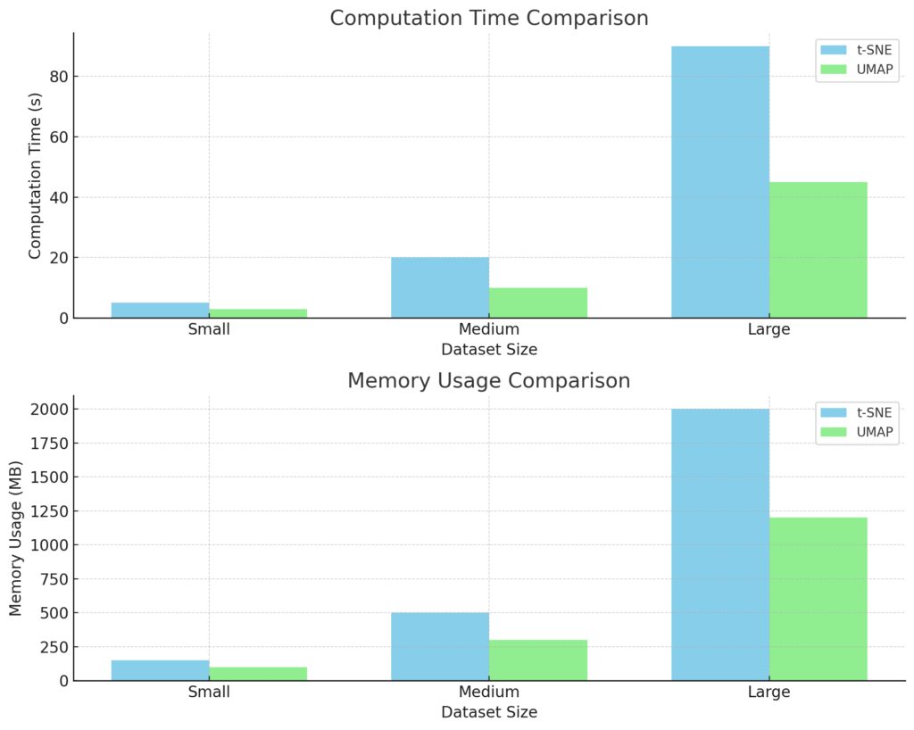
Computation Time: UMAP generally requires less computation time than t-SNE, especially as dataset size increases.
Memory Usage: UMAP also tends to use less memory, making it more efficient for larger datasets.
These insights can help in choosing the appropriate dimensionality reduction method based on dataset size and resource availability.
UMAP, in contrast, is often blazing fast. One of its standout features is its scalability. UMAP is designed to handle large datasets much more efficiently, completing tasks that would take t-SNE hours in just minutes. This makes it a preferred choice for big data applications, where speed can dramatically affect your workflow. If you’re handling large-scale data, UMAP’s faster computational times give it a significant edge over t-SNE.
Handling Large Datasets: Which Method Excels?
When working with massive datasets, t-SNE can start to crumble under the pressure. Due to the way it computes pairwise distances between points, it tends to choke as datasets grow. This doesn’t mean it’s useless for large data—there are approximations of t-SNE that improve speed, like Barnes-Hut t-SNE, but they still don’t match UMAP’s sheer efficiency.

UMAP, on the other hand, shines in this area. With the ability to handle datasets containing millions of points, UMAP’s scalability makes it perfect for high-throughput data, such as genomics, text embeddings, and image data. It can produce results in a fraction of the time, meaning you spend less time waiting and more time interpreting your results.
In short, if you’re working with large datasets, UMAP is the clear winner—faster, more memory-efficient, and more practical when you need to iterate quickly.
Maintaining Global Structure: Who Does It Better?
One of the most common complaints about t-SNE is its inability to preserve the global structure of the data. While t-SNE is amazing at capturing local clusters, it often muddles how these clusters relate to each other on a broader scale. This is fine for cases where only local relationships matter, but it can be limiting when you’re trying to understand overarching trends.
UMAP, however, does a better job of maintaining global structure. It attempts to balance local and global relationships, making it a more well-rounded tool for visualizations where both types of structure are important. For instance, if you want to understand how different categories of images relate to each other, UMAP provides clearer separations between clusters, along with insights into how those clusters connect in a broader sense.
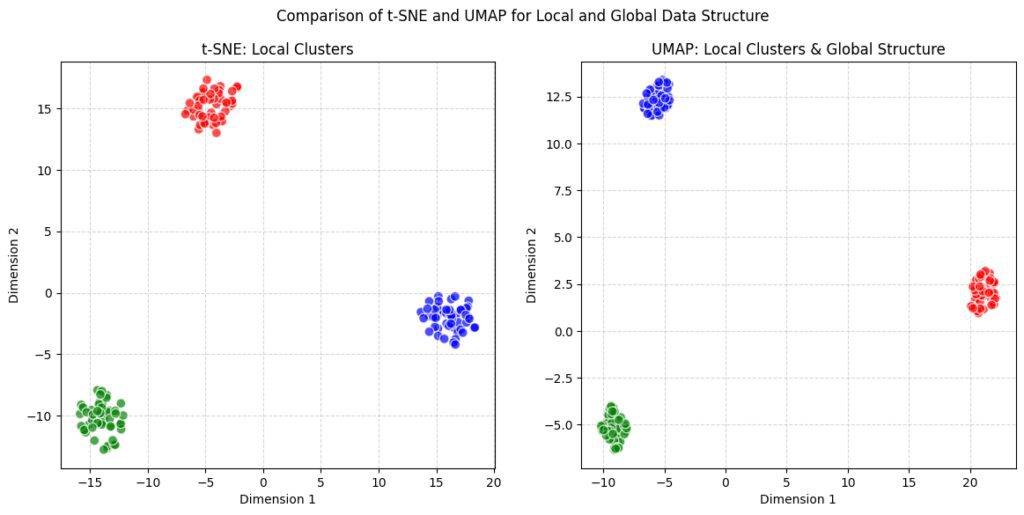
t-SNE: This plot will show clusters based on local similarity, as t-SNE excels at preserving local distances but may distort the global layout.
UMAP: This plot will display local clusters within the context of the global structure, capturing both fine-grained groupings and overall spatial relationships.
While t-SNE tends to produce visualizations where clusters seem disconnected or unrelated, UMAP often shows pathways or transitions between them, giving a better sense of the overall data landscape.
Understanding Local Structure: t-SNE or UMAP?
Even though UMAP offers advantages in global structure, t-SNE still reigns supreme when it comes to capturing local structure. If your primary goal is to understand how points within a cluster relate to one another, t-SNE’s visualizations are hard to beat. It produces beautifully distinct clusters, with tight groupings of related data points, making it ideal for applications like cell clustering in single-cell RNA sequencing or spotting minute patterns in biological data.
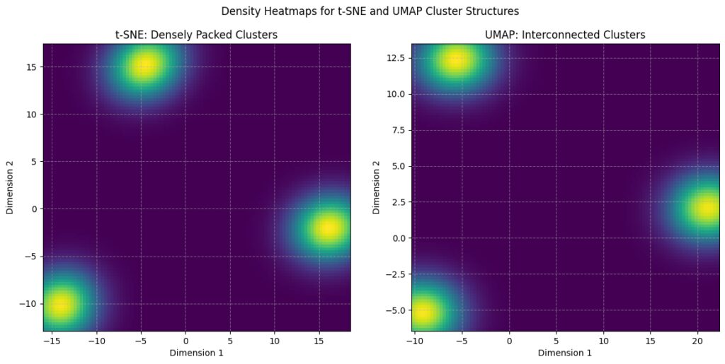
Density Estimation: A Gaussian KDE (Kernel Density Estimate) is used to visualize density.
t-SNE: You’ll see dense, separate clusters with clear boundaries.
UMAP: You’ll see clusters that are more spread out and interconnected, highlighting UMAP’s tendency to maintain more global structure.
UMAP, while maintaining local relationships, can sometimes blur the lines between closely related data points. Its attempt to balance local and global structure means it’s slightly less precise when it comes to very tight clusters, though for many use cases, the difference is negligible.
In short, if you care deeply about understanding local neighborhoods, t-SNE might be the better choice. However, for most real-world applications, UMAP’s broader view without sacrificing too much local structure makes it the more versatile option.
Parameter Tuning: Ease of Use Comparison
Another factor to consider when choosing between t-SNE and UMAP is ease of use—specifically, how much parameter tuning each method requires. t-SNE, while powerful, is notorious for its sensitivity to parameter settings. If you’ve used it, you’ve probably spent time tweaking the perplexity parameter (which controls how t-SNE balances attention between local and global structure) to get the visualization just right.
Not only is it tricky to get right, but changes in parameters can lead to drastically different visualizations. This adds a layer of complexity when trying to interpret results, as a slight tweak can change your entire understanding of the data.
UMAP, by contrast, is often seen as more forgiving when it comes to parameter tuning. While it does have important parameters—like n_neighbors and min_dist—the results tend to be less sensitive to small changes. This makes UMAP more approachable for users who want quick, reliable results without diving deep into parameter adjustments.
In short, if you want an algorithm that “just works” without requiring too much fine-tuning, UMAP tends to be the easier and more user-friendly choice.
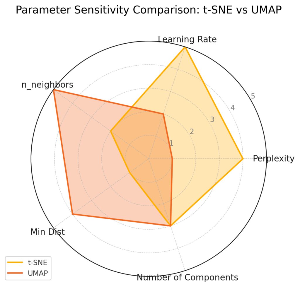
t-SNE shows higher sensitivity to Perplexity and Learning Rate, indicating these parameters significantly influence its behavior.
UMAP displays greater sensitivity to n_neighbors and Min Dist, which are crucial for preserving local and global structures in its dimensionality reduction.
Interpretability of Results: Which One Is Clearer?
When it comes to interpretability, both t-SNE and UMAP have their strengths and weaknesses. However, t-SNE’s results can sometimes be tricky to interpret because of how it emphasizes local structure at the expense of the global picture. As a result, clusters in t-SNE visualizations are often tightly packed, which can make it harder to understand the big-picture context.
If you’ve ever tried to extract high-level insights from a t-SNE plot, you might have found yourself puzzled by how seemingly unrelated clusters sit next to each other.

On the flip side, UMAP often provides a more intuitive sense of the data’s layout. Thanks to its ability to balance local and global relationships, UMAP visualizations are typically easier to read. You get a better sense of the overall structure while still being able to see how individual points group together. This makes UMAP the go-to choice when you need a clear, holistic view of your data’s structure.
That being said, neither method is perfect, and both require a certain degree of subjective interpretation. But if you’re looking for clarity and a more straightforward view, UMAP generally wins out.
Common Applications of t-SNE in Data Science
Despite its drawbacks, t-SNE remains a go-to technique for several specific applications. One of the most famous is in the field of single-cell RNA sequencing (scRNA-seq). t-SNE’s ability to form tight, well-separated clusters makes it ideal for visualizing different cell types in a dataset. Researchers often rely on it to identify new cell types or to spot subtle differences between subpopulations of cells.
Another prominent area where t-SNE shines is in image recognition. When dealing with convolutional neural network (CNN) embeddings, t-SNE helps visualize how image features cluster together, making it easier to see how the model groups similar images. Similarly, natural language processing (NLP) practitioners use t-SNE to visualize word embeddings, revealing how words with similar meanings form groups.
In cases where fine local structure is critical, like identifying tiny variations in biological or image data, t-SNE continues to deliver powerful insights.
Popular Use Cases for UMAP
UMAP, being newer, is rapidly gaining traction across a variety of fields. Its ability to scale to large datasets while maintaining both local and global structure makes it a preferred choice in genomics, where researchers often deal with massive datasets. For instance, UMAP is frequently used for integrating multi-omics data, providing insights into how genetic, proteomic, and other types of data relate to one another.
UMAP’s popularity is also growing in the realm of machine learning for dimensionality reduction before clustering algorithms or visualization. It excels in visualizing high-dimensional embeddings from models like transformers in NLP, giving analysts a clearer picture of how different sentence embeddings relate to one another in space.
In short, UMAP is versatile across disciplines and performs especially well in situations where the dataset is huge, and both local and global structure matter.
When to Choose t-SNE Over UMAP
Though UMAP is gaining popularity, there are still situations where t-SNE is the better choice. If your main goal is to understand fine local structure, such as when working with small, tightly-knit clusters, t-SNE’s precise visualizations can offer more insight than UMAP’s broader approach. For example, in cases where you need to distinguish closely related subpopulations (like in biological datasets), t-SNE may offer better clarity.

Additionally, if you’re already familiar with t-SNE and have a specific perplexity setting that works well for your data, sticking with it might make more sense. Finally, for smaller datasets where computation time isn’t a concern, t-SNE’s detailed local groupings might reveal patterns that UMAP could smooth over.
When UMAP Is the Right Choice
On the flip side, UMAP is often the better choice for large datasets, particularly when you need a method that’s both fast and capable of maintaining global context. If you’re working with millions of points or need to quickly generate visualizations without excessive tuning, UMAP is the go-to. It’s also great for cases where you need to retain global structure, such as in text data embeddings, where understanding how clusters of words or documents relate on a global scale is essential.
Another reason to favor UMAP is its flexibility. With parameters like n_neighbors and min_dist, you can fine-tune the balance between local and global structure, making it adaptable for a wide range of applications, from gene expression data to image processing. If speed, ease of use, and flexibility are top priorities, UMAP is the better fit.
Combining t-SNE and UMAP: Is It Possible?
While t-SNE and UMAP are often seen as competing methods, there’s a growing trend of using them together to leverage their individual strengths. In some cases, researchers start by using UMAP for initial dimensionality reduction due to its speed and ability to handle large datasets, and then follow it up with t-SNE to fine-tune the local relationships.
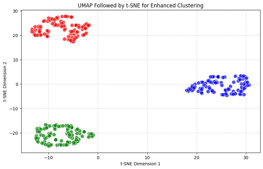
UMAP reduces the data from 10 dimensions to 5, capturing global structure.
t-SNE then reduces the UMAP output to 2 dimensions, focusing on fine-grained clustering.
This combination leverages both UMAP’s global structure preservation and t-SNE’s local clustering capabilities.
This hybrid approach allows you to get the best of both worlds—UMAP provides a broad overview of the data structure, while t-SNE can zoom in on the finer details. For instance, you could run UMAP to get a general sense of clusters and how they relate globally, and then apply t-SNE to zoom in on specific sub-clusters or to further refine the tightness of the local groupings.
Although combining the two methods requires more steps and additional computational time, it can offer deeper insights into complex datasets, especially when both local precision and global structure matter. It’s worth experimenting with if you want to squeeze every possible insight from your data.
Final Thoughts on Dimensionality Reduction Methods
In the t-SNE vs UMAP debate, the right tool depends on the nature of your data and your specific goals. Both algorithms excel at making sense of complex, high-dimensional datasets, but they serve slightly different purposes.
Use t-SNE when you care most about local structure and fine-grained detail. It’s especially helpful for smaller datasets where the computational cost isn’t an issue, or when tight, clear clusters are critical for interpretation. However, keep in mind that t-SNE might require more parameter tuning and patience due to its slower computation time.
On the other hand, UMAP is perfect for those who need a method that balances both local and global structure—especially when dealing with large datasets. Its speed, flexibility, and ease of use make it a fantastic choice for general dimensionality reduction tasks where efficiency and interpretability are key.
Ultimately, both tools have their place in the data scientist’s toolkit, and in many cases, it’s worth trying both to see which provides the clearest insights into your unique dataset.
FAQs: t-SNE vs UMAP
1. What are t-SNE and UMAP used for?
t-SNE (t-Distributed Stochastic Neighbor Embedding) and UMAP (Uniform Manifold Approximation and Projection) are both dimensionality reduction techniques used to visualize high-dimensional data in 2D or 3D. They help reveal patterns, clusters, and relationships in complex datasets.
2. Which method is faster, t-SNE or UMAP?
UMAP is significantly faster than t-SNE, especially with large datasets. UMAP can handle millions of data points efficiently, whereas t-SNE tends to slow down as the dataset grows.
3. Is t-SNE better at capturing local or global structure?
t-SNE excels at preserving local structure. It focuses on keeping similar data points close together in the low-dimensional space. However, it often struggles to maintain global relationships, making it difficult to understand how clusters relate to each other on a broader scale.
4. Does UMAP preserve global structure better than t-SNE?
Yes, UMAP does a better job of maintaining both global and local structure. It balances the relationships between nearby points and how they relate across the entire dataset, making it more suitable for understanding overall patterns.
5. Which one should I use for large datasets?
UMAP is the better choice for large datasets. It’s faster, more scalable, and requires less memory compared to t-SNE. UMAP can handle datasets containing millions of points while still providing meaningful visualizations.
6. Can t-SNE and UMAP be used together?
Yes, t-SNE and UMAP can be combined. One common approach is to use UMAP first for initial dimensionality reduction and then apply t-SNE to further refine the visualization of local clusters. This hybrid method leverages the strengths of both techniques.
7. How sensitive are t-SNE and UMAP to parameter settings?
t-SNE can be very sensitive to parameters like perplexity, which can significantly alter the resulting visualization. In contrast, UMAP is generally more forgiving, though parameters like n_neighbors and min_dist still influence the output. UMAP often requires less fine-tuning overall.
8. Which method is more interpretable?
UMAP often produces more interpretable visualizations because it preserves both local and global structure. t-SNE can create tightly packed clusters, which may make it harder to interpret how different clusters relate to each other.
9. Can I use t-SNE or UMAP for non-visualization purposes?
Yes, while t-SNE and UMAP are often used for visualization, they can also be used for preprocessing before clustering or classification tasks by reducing the number of features in a dataset. UMAP is particularly useful in this regard due to its efficiency and flexibility.
10. What are some common applications of t-SNE?
t-SNE is commonly used in single-cell RNA sequencing, image recognition, and word embeddings in natural language processing. It’s well-suited for scenarios where understanding small, local clusters of data is critical.
11. What are popular use cases for UMAP?
UMAP is widely used in genomics, large-scale image data, text embeddings, and multi-omics data. It’s favored for large datasets where both local and global data structure need to be preserved.
12. Is t-SNE harder to tune than UMAP?
Yes, t-SNE typically requires more careful parameter tuning, especially with the perplexity setting, which can drastically affect the visualization. UMAP, while it also has important parameters, tends to be easier to use with less need for extensive tuning.
13. Does t-SNE or UMAP work better for imbalanced datasets?
UMAP tends to handle imbalanced datasets better than t-SNE because of its ability to maintain global structure while still clustering similar points together. t-SNE may produce misleading visualizations in highly imbalanced datasets, as it emphasizes local structure without considering the global context.
14. Which method should I use for small datasets?
For small datasets, t-SNE can be a good choice. Its ability to form distinct, tight clusters can provide valuable insights when you don’t need to worry about computational speed or scalability. However, UMAP still remains a competitive option due to its speed and flexibility, even on smaller datasets.
Useful Resources for Learning About t-SNE and UMAP
- Scikit-Learn Documentation:
- Both t-SNE and UMAP are available as part of the Scikit-learn library. Their official documentation provides explanations of the algorithms, implementation details, and examples.
- t-SNE: Scikit-learn t-SNE Documentation
- UMAP: UMAP Documentation
- UMAP GitHub Repository:
- The official UMAP implementation on GitHub, with a variety of tutorials and explanations about how UMAP works under the hood.
- UMAP GitHub Repository
- “How to Use t-SNE Effectively” by Distill.pub:
- This interactive article provides an in-depth guide on t-SNE, including how to tune parameters like perplexity and how to interpret visualizations.
- UMAP vs t-SNE Comparison by Towards Data Science:
- A well-written blog post that compares t-SNE and UMAP, discussing their respective strengths, weaknesses, and when to use one over the other.
- “Dimensionality Reduction in Python: PCA, UMAP, and t-SNE” by Analytics Vidhya:
- A step-by-step guide to using these dimensionality reduction techniques, with Python code examples and explanations on how to apply them in different scenarios.
- Comprehensive UMAP Guide by PyData:
- A technical talk explaining UMAP in detail, including its theoretical background, performance comparison with t-SNE, and real-world use cases.
- UMAP: Uniform Manifold Approximation and Projection
- Python Data Science Handbook by Jake VanderPlas:
- A great book that explains t-SNE and UMAP in the context of data science, with clear examples using Python.
- Python Data Science Handbook
- “Visualizing t-SNE and UMAP” by Nature Methods:
- This article discusses how t-SNE and UMAP are used in biological data analysis, particularly in high-dimensional data like single-cell RNA sequencing.
- Visualizing High-Dimensional Data
- Google Colab Notebooks for Hands-On Practice:
- For those who prefer a more hands-on approach, here are two Google Colab notebooks to practice using t-SNE and UMAP:
- t-SNE: Google Colab t-SNE Notebook
- UMAP: Google Colab UMAP Notebook
- “A Practical Guide to t-SNE and UMAP for Data Visualization” by DataCamp:
- This guide gives a practical overview on how to use t-SNE and UMAP in Python, complete with code snippets and examples of when to use each method.
