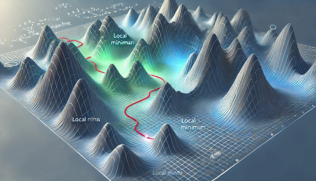
Optimization challenges often emerge in training neural networks, especially when models get “stuck” in local minima. While local minima might offer decent solutions, they can hinder the model from reaching optimal performance.
This article explores effective techniques and tools to help neural networks escape these traps, resulting in faster and more accurate training.
Understanding Local Minima in Neural Networks
What are Local Minima in Optimization?
In the context of neural networks, a local minimum is a point in the loss landscape where the loss is lower than nearby points but not the lowest possible. Neural networks often have highly complex, non-convex loss surfaces filled with hills, valleys, and flat areas. Thus, they can easily get “trapped” in a local minimum, halting further progress in model training.
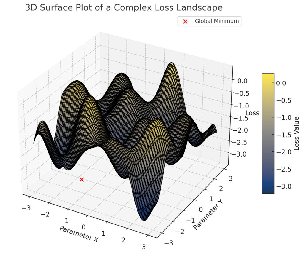
Valleys are represented by darker regions, indicating lower loss values.
Peaks appear lighter, representing higher loss values.
Global Minimum: A prominent, deep global minimum is highlighted in red, deeper than any local minimum.
This visualization demonstrates the challenge of navigating through local minima and saddle points in neural network optimization, with the global minimum as the target in the landscape.
Local minima issues especially affect deep and complex networks, which can suffer from long training times and convergence to suboptimal performance. Escaping these areas can boost accuracy and reduce training costs.
Why Local Minima Are Problematic
Local minima are problematic because they prevent the network from finding the global minimum—the point where the loss is the lowest across the entire landscape. This can result in:
- Suboptimal model performance, as the weights settle on less effective configurations.
- Increased resource consumption as training stalls.
- Difficulty in reaching desired accuracy, especially for deep learning tasks like image recognition or natural language processing.
Avoiding or escaping local minima is crucial for high-performing models and faster training times.
Gradient-Based Techniques for Escaping Local Minima
Momentum-Based Optimization
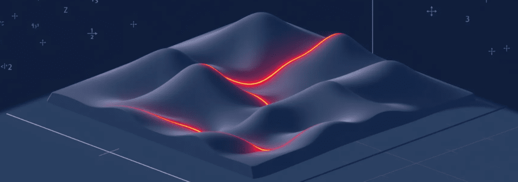
Momentum optimization modifies gradient descent by adding a fraction of the previous update to the current update. This allows the algorithm to push through small local minima by “building up speed.”
Momentum algorithms achieve this by accumulating previous gradients, which helps the model traverse small valleys and avoid settling. Popular momentum-based optimizers include:
- SGD with Momentum: Introduces a momentum factor to vanilla SGD, improving speed and accuracy.
- Nesterov Accelerated Gradient (NAG): Uses a look-ahead step to anticipate gradients, often better for faster convergence.
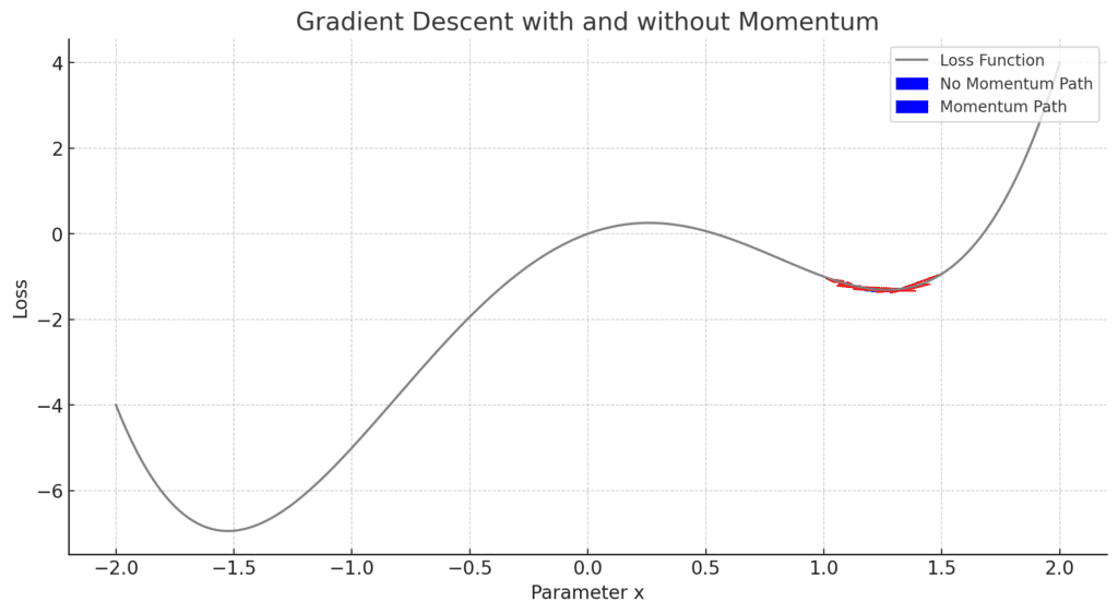
Blue Arrows: The path without momentum, showing slower convergence and more difficulty overcoming local minima.
Red Arrows: The path with momentum, which accelerates down slopes and moves through local minima more effectively, converging faster toward lower loss regions.
This visualization highlights how momentum helps overcome shallow minima and saddle points, improving convergence toward a global minimum.
Adaptive Learning Rates
Using an adaptive learning rate helps the model avoid getting stuck by adjusting the step size during training. Adaptive optimizers dynamically change the learning rate based on gradient information, making it easier to escape local minima.
Popular adaptive learning rate optimizers include:
- Adam: Adjusts the learning rate based on past gradients, balancing between speed and stability.
- Adagrad and RMSprop: Tailor the learning rate based on gradient magnitude, which helps with irregular loss landscapes.
These optimizers offer a balance between speed and accuracy, and their adaptability can help neural networks avoid local minima.
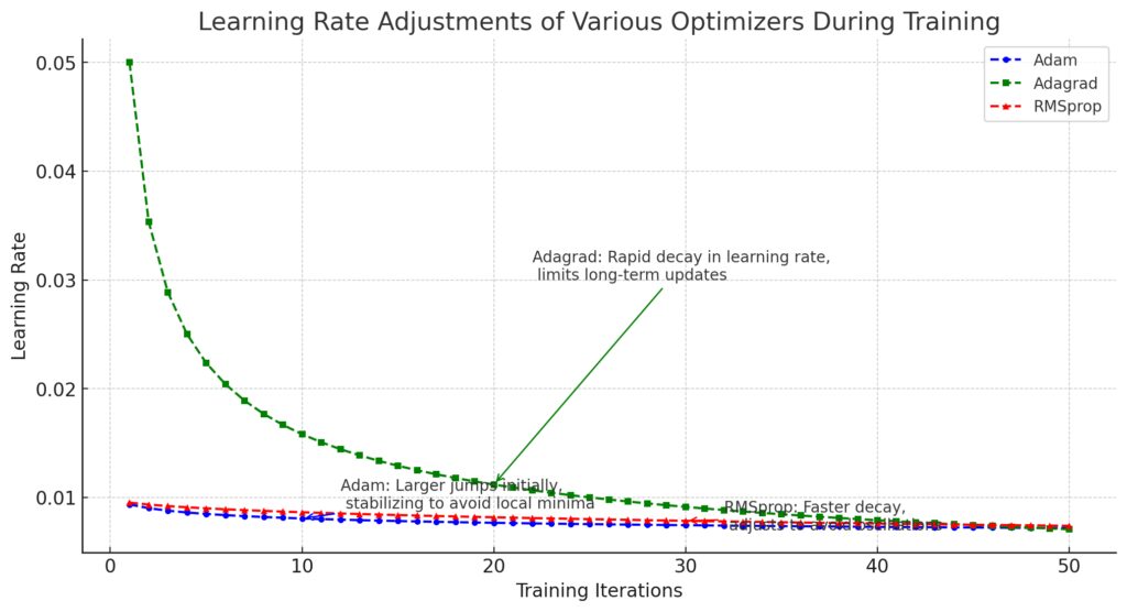
Adam (blue): Begins with larger jumps, allowing the model to escape local minima, then gradually stabilizes the learning rate as training progresses.
Adagrad (green): Rapidly decays its learning rate, which helps with initial adjustments but limits further updates over time.
RMSprop (red): Uses a more aggressive decay than Adam to prevent oscillations, with slightly larger initial jumps that taper off.
Randomization Techniques to Aid Optimization
Adding Noise to the Gradients
Adding random noise to gradients can “shake up” the weights, helping them escape local minima. This method, also known as stochastic gradient descent (SGD), prevents the model from settling prematurely and explores a broader area of the loss landscape.
This technique is commonly used in mini-batch training, where the randomness of smaller batches introduces variability in gradient calculations. This variability has the side benefit of pushing the model out of local minima.
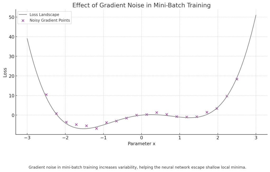
Gray Curve: Represents the loss landscape, with visible local minima.
Purple Points: Indicate noisy gradient points where random disturbances push values away from local minima.
Illustrating how gradient noise increases variability, aiding the neural network in escaping shallow local minima and exploring a broader section of the loss landscape to converge on the global minimum.
Dropout for Regularization
Dropout is primarily a regularization technique to prevent overfitting, but it can also help in escaping local minima. By randomly “dropping” units (i.e., setting their output to zero), dropout introduces randomness that forces the model to rely on different pathways during each forward pass.
This randomness helps in exploring different neural pathways, pushing the model away from local minima and encouraging a more generalized solution.
Advanced Methods for Escaping Local Minima

Simulated Annealing
Simulated annealing is inspired by the metallurgical process where materials are slowly cooled to eliminate defects. In neural network optimization, simulated annealing involves gradually lowering the “temperature” (or randomness) as training progresses, allowing the model to escape local minima in early stages and settle into a global minimum as the “temperature” decreases.
Implementing simulated annealing can be more challenging but effective for highly non-convex optimization landscapes.
Gradient Clipping to Control Gradient Magnitude
How Gradient Clipping Works
Gradient clipping is a technique used to prevent gradients from becoming excessively large during training. By setting a maximum threshold for gradient values, this method ensures that the updates remain within a manageable range. This can help with stability, particularly in recurrent neural networks (RNNs), where large gradients are common.
When gradients are kept in check, they are less likely to push the model into steep, narrow local minima. Gradient clipping can also reduce issues related to vanishing and exploding gradients, two challenges that often appear in training deep networks.
Implementing Gradient Clipping in Popular Frameworks
Popular deep learning frameworks like TensorFlow and PyTorch have built-in support for gradient clipping. Here’s how you can add it to your model training loop:
- In PyTorch, use
torch.nn.utils.clip_grad_norm_to clip gradients within a specified norm. - In TensorFlow, apply
tf.clip_by_valueortf.clip_by_normto limit gradient values within a defined range.
Using gradient clipping adds stability to training and can keep the model from overshooting or undershooting in complex landscapes.
Leveraging Ensembles and Multiple Initializations

Why Multiple Initializations Help
Initializing weights from different starting points can prevent the model from falling into the same local minima each time. By training multiple models with different initializations, or training one model with different initializations and picking the best outcome, you increase the chances of escaping suboptimal solutions.
This approach is often used in ensemble learning, where multiple models with different initializations are combined for improved predictions. Ensemble models help “smooth out” the decision boundary and improve performance by capturing a broader range of patterns.
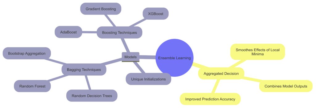
Models: Trained through different techniques:Unique Initializations: Models start with varying initial conditions.
Bagging Techniques: Includes Random Decision Trees, Random Forests, and Bootstrap Aggregation.
Boosting Techniques: Covers AdaBoost, Gradient Boosting, and XGBoost.
Aggregated Decision: Combines model outputs to smooth out local minima effects and improve prediction accuracy.
Using Bagging and Boosting
Bagging and boosting are two techniques in ensemble learning that benefit from multiple initializations:
- Bagging: Randomly samples data subsets for each model, reducing variance and aiding in model stability.
- Boosting: Sequentially trains models, correcting previous mistakes, which helps the ensemble escape local minima by adjusting for errors.
Combining ensemble models can offer better generalization and robustness compared to a single network, making them valuable for escaping optimization traps.
Metaheuristic Algorithms for Improved Convergence
Genetic Algorithms
Genetic algorithms (GAs) take inspiration from biological evolution, using “mutations” and “crossovers” to explore various regions of the loss landscape. GAs can effectively search for better solutions by introducing diversity into model parameters, reducing the chance of falling into local minima.
Genetic algorithms are typically applied to specific layers or weights rather than the entire network, making them a unique but powerful tool for highly complex or sparse optimization landscapes.

Initialization: Begin with a randomly generated population of neural network parameters.
Selection: Choose the fittest individuals based on evaluation.
Crossover: Combine selected individuals to create offspring.
Mutation: Introduce random variations to escape local minima.
Replacement and Termination: Replace the population and check for convergence.
Mutation is highlighted as a crucial step to add diversity, helping avoid local minima traps.
Particle Swarm Optimization (PSO)
Particle Swarm Optimization (PSO) simulates the behavior of a swarm (like a flock of birds) to locate optimal regions in a loss landscape. Each particle in the swarm represents a potential solution and “flies” through the space, adjusting its position based on both personal and global best positions.
PSO works well in combination with traditional optimizers, such as Adam or SGD, by helping to identify promising areas and escape local minima. It’s most effective when used intermittently during training rather than in every update.
Software Tools to Aid in Escaping Local Minima

TensorFlow and Keras for Flexible Optimizer Integration
TensorFlow and its high-level API, Keras, are robust tools that make it easy to experiment with various optimization techniques. Both offer built-in optimizers like Adam, SGD with momentum, RMSprop, and Adagrad, which are all adaptive optimizers that can help avoid local minima.
Keras also allows you to add custom callbacks, making it easy to incorporate additional randomization or regularization. For example:
- Learning Rate Scheduler: This callback adjusts the learning rate over epochs, allowing the model to “shake off” local minima in early stages and settle later on.
- Custom Callbacks: Keras lets you implement custom callbacks, like adding noise to gradients or adjusting dropout rates during training, which can encourage more diverse training paths.
For those working in TensorFlow, TensorBoard is an essential tool. Its visualization capabilities make it easier to monitor gradient behavior, which can indicate when local minima might be an issue.
PyTorch for Customization and Advanced Techniques
PyTorch is known for its flexibility, making it a favorite among researchers experimenting with custom optimization techniques. PyTorch’s dynamic computation graph allows for more intricate adjustments during training, and the framework offers several helpful modules:
- Gradient Clipping: Easily add gradient clipping with
torch.nn.utils.clip_grad_norm_. - Custom Optimizers: PyTorch’s optimizer API is extensible, so you can modify existing optimizers or create new ones. This can be useful for implementing advanced techniques like simulated annealing or genetic algorithms.
With PyTorch’s flexibility, users can implement and test novel approaches to escape local minima, such as combining ensemble models with dropout for robustness.
Hyperparameter Optimization with Optuna
Optuna is a hyperparameter optimization framework designed for efficient exploration of hyperparameter space. By running automated trials, Optuna helps find parameter configurations that can make a difference in escaping local minima.
Optuna’s advanced sampling and pruning strategies make it ideal for optimizing neural networks. For example:
- Learning Rate Tuning: Adjusting learning rates at different stages of training can prevent models from converging too early.
- Batch Size and Dropout Rate Tuning: These parameters can introduce the necessary variance in training that helps avoid local minima.
Optuna integrates well with both TensorFlow and PyTorch, making it a valuable tool in any neural network pipeline.
Ray Tune for Distributed Hyperparameter Tuning
For large-scale projects, Ray Tune is a distributed hyperparameter tuning library that works well for optimizing deep learning models. Ray Tune provides seamless integration with both PyTorch and TensorFlow and is designed to scale across multiple GPUs and nodes.
Ray Tune offers several unique features that can help with local minima issues:
- Bayesian Optimization: A probabilistic approach to explore the best hyperparameters, helping the model find optimal learning paths.
- Early Stopping and Pruning: Automatically terminates low-performing trials, saving time and focusing on promising configurations.
By distributing the tuning process, Ray Tune provides a powerful way to find configurations that may avoid local minima while optimizing performance across a broad parameter space.
In summary, overcoming local minima in neural network training requires a combination of optimization techniques and smart software tools. Whether you’re using adaptive optimizers, gradient clipping, ensemble learning, or advanced metaheuristic approaches like genetic algorithms and particle swarm optimization, the right strategy can significantly improve model performance. Tools like TensorFlow, PyTorch, Optuna, and Ray Tune provide a practical, flexible foundation for implementing these techniques and ensuring your model reaches its full potential.
FAQs
How do local minima impact neural network performance?
Local minima can prevent neural networks from reaching the best possible performance by trapping them in suboptimal solutions. This results in higher error rates and limits the model’s accuracy, especially on complex tasks. Getting out of local minima is essential for more efficient training and better generalization to unseen data.
What is gradient clipping, and how does it help in training?
Gradient clipping restricts the size of gradients during backpropagation to prevent them from becoming excessively large. This stabilizes training, especially for deep and recurrent networks, and helps avoid both exploding and vanishing gradient issues. By managing gradient magnitudes, it also reduces the chance of the model getting stuck in steep local minima.
Why are adaptive optimizers useful for escaping local minima?
Adaptive optimizers like Adam and RMSprop adjust the learning rate dynamically based on the gradients, making training more resilient to getting stuck. By increasing the learning rate when necessary, these optimizers help the model explore different regions of the loss landscape, aiding in moving past local minima for faster convergence.
How can dropout help with local minima in neural networks?
Dropout randomly disables neurons during training, forcing the model to rely on multiple neural pathways. This introduces a form of randomness that helps avoid settling in specific local minima. Dropout also acts as regularization, improving the model’s ability to generalize and reducing the risk of overfitting.
What’s the role of random noise in escaping local minima?
Adding noise to gradients introduces variation that can push the model out of small local minima. This randomness helps the model explore a broader range of values, increasing the chances of finding a path to a better global minimum. Stochastic gradient descent (SGD), for instance, leverages this randomness, especially in mini-batch training.
Can hyperparameter tuning improve optimization in neural networks?
Yes, hyperparameter tuning helps find configurations that may avoid local minima by exploring a wide range of parameter values. Tools like Optuna and Ray Tune automate this process, helping identify optimal learning rates, batch sizes, and dropout rates to ensure better training outcomes and faster convergence.
How do genetic algorithms and particle swarm optimization assist in neural network training?
Genetic algorithms and particle swarm optimization (PSO) are metaheuristic techniques that explore diverse regions of the loss landscape. Genetic algorithms evolve the best solutions over generations, while PSO simulates a swarm of solutions moving towards optimal points. Both techniques are effective at breaking free from local minima, especially in complex, non-convex optimization landscapes.
Which frameworks support advanced optimization techniques for neural networks?
TensorFlow and PyTorch are the primary frameworks for neural networks, offering flexibility to implement adaptive optimizers, gradient clipping, and custom training functions. Both frameworks integrate with hyperparameter tuning tools like Optuna and Ray Tune for streamlined optimization and tuning at scale, making them ideal for tackling local minima issues in neural networks.
What is the difference between local minima and saddle points?
In neural network optimization, a local minimum is a point where the loss is lower than in the immediate surrounding area but not necessarily the lowest possible (global minimum). A saddle point, on the other hand, has a lower loss than points along some directions but not others, meaning it’s a “flat” area with no distinct upward or downward trend. Neural networks are more likely to encounter saddle points than true local minima, and they can slow down training because gradients become small, making it hard to move away.
How does simulated annealing work in neural network optimization?
Simulated annealing is an optimization technique inspired by the cooling process in metalwork, where the material is gradually cooled to reach a stable state. In neural networks, simulated annealing involves introducing random fluctuations to the learning rate or weights in early training stages, then reducing randomness as training progresses. This helps the model explore various regions of the loss landscape early on and settle into a better minimum over time, reducing the risk of local minima trapping.
Is batch size important for escaping local minima?
Yes, batch size can play a significant role in escaping local minima. Smaller batch sizes introduce more noise into gradient calculations, making it easier for the model to explore and potentially escape small local minima. However, if the batch size is too small, it may slow down convergence. Mini-batch gradient descent is a commonly used compromise, offering both speed and a degree of randomness that helps in avoiding local minima.
What are ensemble models, and how do they help in avoiding local minima?
Ensemble models combine the predictions of multiple models trained with different initializations, architectures, or subsets of data. By aggregating results, ensembles can “smooth out” predictions and improve overall accuracy, helping to mitigate the impact of local minima that individual models might encounter. Techniques like bagging and boosting are used to build ensembles, making them effective for both performance improvements and avoiding local traps.
Why are weight initializations important in avoiding local minima?
Weight initialization defines the starting point for neural network parameters, and different initializations can lead to different local minima. Effective initializations, such as He initialization for ReLU-based networks or Xavier initialization for sigmoid activations, help start the model closer to promising areas of the loss landscape. This reduces the chance of getting stuck in poor local minima and can speed up convergence.
How do second-order optimization methods compare to first-order methods in terms of local minima?
Second-order methods, like the Newton method or BFGS, use information from the second derivative (Hessian matrix) to find optimal points, unlike first-order methods like gradient descent that rely only on the first derivative. Second-order methods are more effective at escaping saddle points and shallow local minima but are computationally expensive for large neural networks. As a result, they’re less commonly used in deep learning but are valuable in smaller models or specific layers of complex architectures.
What role does regularization play in avoiding local minima?
Regularization techniques like L2 regularization and dropout help reduce overfitting by penalizing large weight values and enforcing sparsity in the network. Regularization discourages the model from fitting too closely to training data, which can sometimes cause it to get stuck in local minima. By preventing overfitting, regularization encourages the model to find smoother, more generalized loss landscapes, making it easier to avoid and escape local minima.
Can visualizing the loss landscape help in understanding local minima issues?
Yes, visualizing the loss landscape can provide insights into local minima and other topographical challenges the model may face. Tools like TensorBoard and loss landscape visualization libraries allow you to plot the loss function across different dimensions, making it easier to see areas where the model may be getting stuck. Visualization can guide adjustments to model architecture or optimization techniques to better navigate complex landscapes and reach lower minima.
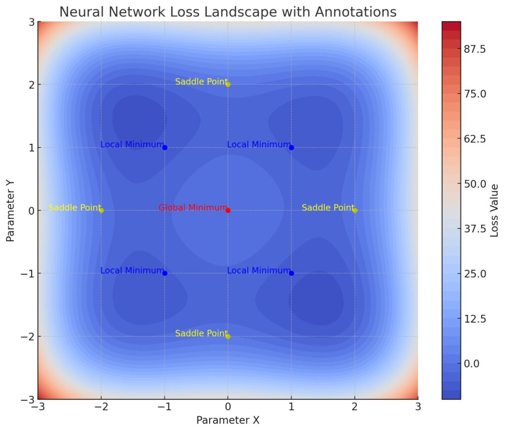
Color Gradient: Ranges from darker regions (lower loss) to lighter regions (higher loss), helping to visualize the terrain.
Global Minimum (Red Dot): The optimal point in the loss landscape.
Saddle Points (Yellow Dots): Points where optimizers may oscillate, representing challenging areas during training.
Local Minima (Blue Dots): Shallow minima where optimizers may get stuck, impacting convergence.
This visualization emphasizes how variations in the loss landscape, such as saddle points and local minima, create potential training obstacles, illustrating the complexities optimizers must navigate to find the global minimum.
Resources
Software and Libraries
- TensorFlow and Keras
Both TensorFlow and Keras offer flexible tools for implementing advanced optimizers, gradient clipping, and custom training loops. Keras’s ease of use with optimizers and TensorFlow’s visualization features make them ideal for tracking and optimizing models. Visit TensorFlow for documentation. - PyTorch
Known for flexibility, PyTorch is widely used for custom optimization experiments. Its dynamic graphing and support for custom optimizers make it ideal for testing novel approaches to local minima issues. Visit PyTorch for resources and tutorials. - Optuna
This hyperparameter optimization library is useful for automating parameter searches, making it easier to find configurations that avoid local minima. It integrates with both TensorFlow and PyTorch. Available at Optuna.org. - Ray Tune
Ray Tune is a powerful tool for distributed hyperparameter optimization, suited for large-scale experiments. It supports Bayesian optimization, early stopping, and other features that help neural networks avoid local minima. Visit Ray.io for documentation.