
XGBoost is an incredibly powerful machine learning algorithm, but to unlock its full potential, you need to master hyperparameter tuning.
Properly tuning the hyperparameters can significantly improve model performance by optimizing the trade-off between bias and variance.
In this guide, we’ll explore the most important hyperparameters to adjust, how they impact your model, and practical techniques to help you find the best settings.
What Are Hyperparameters in XGBoost?
Hyperparameters in XGBoost are settings that control how the algorithm learns from the data. These parameters are set before training begins and directly affect the model’s behavior, such as the complexity of the trees, learning rate, and regularization.
Unlike model parameters (weights or splits), hyperparameters are not learned from the data during training—they need to be manually specified or tuned through experiments.
Why Hyperparameter Tuning Matters
Hyperparameter tuning in XGBoost is essential because it can:
- Prevent overfitting or underfitting by controlling model complexity.
- Optimize model accuracy by finding the ideal balance between learning speed and model depth.
- Speed up training time by efficiently using computational resources like memory and CPU/GPU.
Poorly set hyperparameters can lead to poor generalization, where your model performs well on training data but fails on unseen data. Tuning ensures your model performs consistently across both.
Key Hyperparameters in XGBoost
Here are the most important hyperparameters you’ll want to focus on when tuning your XGBoost model. We’ll break them down by function and provide practical guidelines for adjusting each one.
1. Learning Rate (eta)
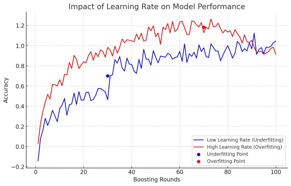
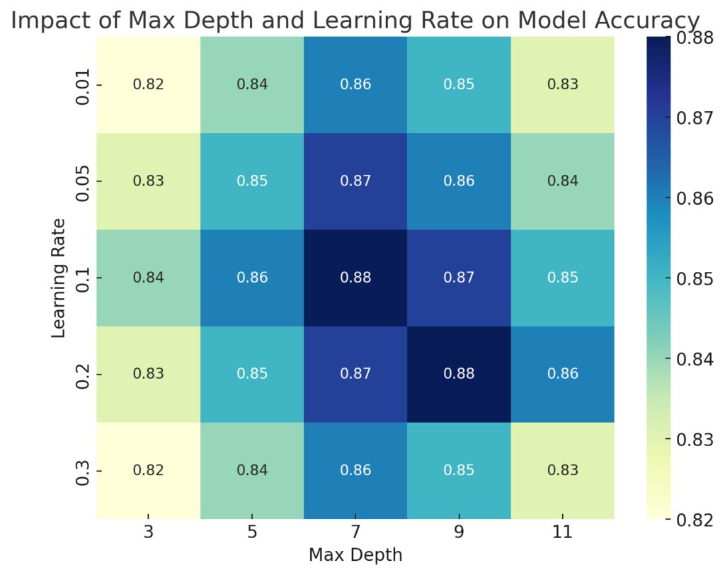
The learning rate controls how much the model adjusts with each boosting round. A smaller learning rate will slow down the learning process but generally leads to a more accurate model, while a large learning rate can make the model converge quickly, at the risk of overshooting.
- Default: 0.3
- Range: 0.01 to 0.3
- Tip: Start with a lower learning rate (e.g., 0.05 or 0.1) and increase the number of boosting rounds to compensate.
2. Number of Trees (n_estimators)
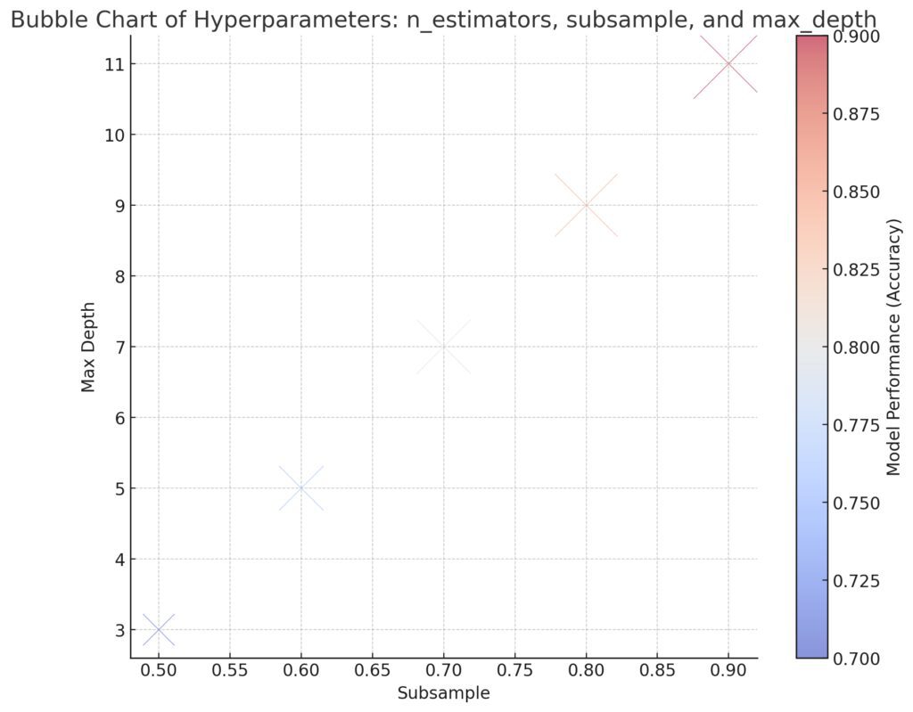
This parameter defines how many trees (boosting rounds) the algorithm will build. More trees can improve performance, but too many trees can cause overfitting, especially if the learning rate is too high.
- Default: 100
- Range: 100 to 1000
- Tip: Start with a moderate number of trees and combine it with a lower learning rate for better results.
3. Max Depth (max_depth)
Max depth controls how deep each tree grows. Deeper trees capture more complex patterns but can also lead to overfitting. Shallow trees are more likely to underfit but are faster to train.
- Default: 6
- Range: 3 to 10
- Tip: For most applications, a max depth between 3 and 8 works well. Start with a value of 6 and adjust based on performance.
4. Subsampling (subsample)
The subsample parameter refers to the fraction of the training data used to grow each tree. Using a subsample less than 1.0 can help prevent overfitting by adding randomness to the training process.
- Default: 1.0
- Range: 0.5 to 1.0
- Tip: Try subsample values between 0.6 and 0.9 for better generalization.
5. Colsample_bytree (colsample_bytree)
This parameter controls the fraction of features used to train each tree. Reducing the number of features per tree can help reduce overfitting, particularly in high-dimensional datasets.
- Default: 1.0
- Range: 0.3 to 1.0
- Tip: Values between 0.5 and 0.9 work well in most cases, depending on the dataset’s dimensionality.
6. Gamma (gamma)
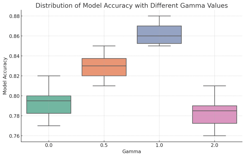
Gamma controls whether a tree node will be split based on the reduction in loss after the split. Higher values lead to more conservative tree growth, which helps combat overfitting.
- Default: 0
- Range: 0 to 5
- Tip: Set gamma to values between 0 and 1 for most tasks. Increase it if you notice overfitting.
7. L1 and L2 Regularization (alpha and lambda)
- L1 Regularization (alpha): Encourages sparsity in the model by applying penalties to the absolute values of weights.
- L2 Regularization (lambda): Prevents overly large weights by applying penalties to their squares.
Both help control model complexity, making it less likely to overfit.
- Default:
alpha= 0,lambda= 1 - Range:
alpha: 0 to 1,lambda: 0 to 10 - Tip: Start with the default values. If your model overfits, consider increasing these parameters.
8. Min Child Weight (min_child_weight)
This parameter defines the minimum sum of instance weights required to create a new leaf node. Higher values prevent the model from learning overly specific patterns that could lead to overfitting.
- Default: 1
- Range: 1 to 10
- Tip: Start with a value between 1 and 5. Increase it if your model overfits.
9. Tree Method (tree_method)
This determines the method used for constructing trees. XGBoost offers different options depending on your dataset size and available hardware.
- Default:
"auto" - Options:
"exact","approx","hist","gpu_hist" - Tip: Use
"gpu_hist"if you’re training on a GPU. For large datasets,"hist"works faster than"exact".
Techniques for Hyperparameter Tuning
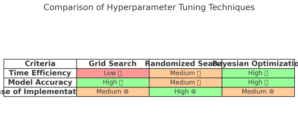
1. Grid Search
Grid Search is a brute-force method where you specify a range of values for each hyperparameter, and the algorithm tries every possible combination. While effective, grid search can be computationally expensive.
- Pros: Exhaustive, ensures you find the best hyperparameters.
- Cons: Slow, especially with many hyperparameters or large datasets.
from sklearn.model_selection import GridSearchCV
import xgboost as xgb

param_grid = {
    'max_depth': [3, 5, 7],
    'learning_rate': [0.01, 0.1, 0.2],
    'n_estimators': [100, 200, 300],
}

xgb_model = xgb.XGBClassifier()
grid_search = GridSearchCV(estimator=xgb_model, param_grid=param_grid, cv=3, scoring='accuracy')
grid_search.fit(X_train, y_train)
2. Randomized Search
Randomized Search randomly selects combinations of hyperparameters from a predefined range. It’s faster than grid search and works well with a large number of hyperparameters.
- Pros: Efficient, good performance with fewer iterations.
- Cons: May miss the best combination.
from sklearn.model_selection import RandomizedSearchCV
import xgboost as xgb

param_dist = {
    'max_depth': [3, 5, 7, 10],
    'learning_rate': [0.01, 0.05, 0.1],
    'n_estimators': [100, 200, 500],
    'subsample': [0.6, 0.8, 1.0],
}

xgb_model = xgb.XGBClassifier()
random_search = RandomizedSearchCV(estimator=xgb_model, param_distributions=param_dist, n_iter=50, scoring='accuracy', cv=3)
random_search.fit(X_train, y_train)
3. Bayesian Optimization
Bayesian Optimization uses past results to make educated guesses about the next best set of hyperparameters to try. It’s more efficient than both grid and random search, especially when you’re working with expensive or time-consuming models.
- Pros: More efficient, better performance in fewer trials.
- Cons: More complex to implement.
Libraries like Hyperopt or Optuna are great for performing Bayesian optimization in Python.
Conclusion: Fine-Tuning for Success
Hyperparameter tuning is essential for getting the most out of your XGBoost model. By carefully adjusting parameters like learning rate, max depth, and regularization, you can significantly boost your model’s performance and make it more robust. Start with simple tuning techniques like grid or random search, and as you become more familiar with the algorithm, try advanced methods like Bayesian optimization.
Tuning may seem like a daunting task, but it’s a critical step toward building machine learning models that excel in both accuracy and efficiency.
Further Reading
FAQs
Why is learning rate important in XGBoost?
The learning rate controls how much the model learns with each boosting round. A lower learning rate makes learning more gradual, leading to a potentially more accurate model, while a higher learning rate speeds up training but increases the risk of overfitting.
How do I choose the number of trees (n_estimators)?
The number of trees (n_estimators) depends on the complexity of the problem and the learning rate. More trees generally increase accuracy, but too many can cause overfitting. A low learning rate often requires a higher number of trees to maintain accuracy.
What does max depth control in an XGBoost model?
Max depth controls the complexity of each tree in XGBoost. A deeper tree captures more complex patterns but can lead to overfitting. A shallower tree is faster to train and may prevent overfitting, but it might miss subtle patterns.
How does XGBoost handle missing values?
XGBoost can automatically handle missing values by learning the best direction to take when encountering a missing value during training. This feature simplifies data preprocessing, as you don’t need to impute missing data manually.
What is the difference between L1 and L2 regularization in XGBoost?
L1 regularization (alpha) adds a penalty to the absolute value of the weights, encouraging a sparser model. L2 regularization (lambda) penalizes the squared value of the weights, reducing overly large coefficients. Both are used to prevent overfitting and make the model more generalizable.
Can XGBoost be used with GPU support?
Yes, XGBoost supports GPU acceleration, which can significantly speed up training for large datasets. Setting the tree_method parameter to "gpu_hist" enables GPU support, leveraging parallel computation for faster results.
What is subsample and how does it affect the model?
Subsample controls the fraction of training data used to build each tree. Lower values introduce more randomness, helping prevent overfitting by making the model less sensitive to individual samples. A value between 0.6 and 0.9 is commonly used for generalization.
How do I know if my XGBoost model is overfitting?
Overfitting occurs when your model performs well on training data but poorly on test data. Signs of overfitting include a significant gap between training and validation scores. Adjust parameters like max_depth, subsample, and increase regularization to mitigate overfitting.
What is gamma in XGBoost?
Gamma determines the minimum loss reduction required to make a split. Higher gamma values make the model more conservative, only allowing splits that significantly reduce the error, which helps to combat overfitting.
How does Bayesian Optimization work for hyperparameter tuning?
Bayesian Optimization uses past evaluations to inform the next choice of hyperparameters, making it more efficient than random or grid search. It aims to find the optimal set of hyperparameters using fewer iterations, saving time and computational resources.
Which hyperparameter tuning technique is best for XGBoost?
The best technique depends on your data and computational resources. Grid Search is exhaustive but slow, Randomized Search is faster but less precise, and Bayesian Optimization is efficient, making it ideal for complex or time-consuming models.
How can I visualize the results of hyperparameter tuning?
You can visualize the results of hyperparameter tuning using plots, such as heat maps for accuracy, learning curves, or feature importance plots. These visualizations can help you understand the impact of each parameter and guide further adjustments.
What does colsample_bytree do in XGBoost?
Colsample_bytree controls the fraction of features (columns) that XGBoost uses to train each tree. Reducing the number of features can help prevent overfitting and reduce training time. It adds randomness to the model, leading to better generalization on unseen data.
Is feature scaling necessary when using XGBoost?
No, feature scaling (like normalization or standardization) is not required for XGBoost because it uses decision trees. Unlike linear models, decision trees are not sensitive to the scale of input features, which makes XGBoost a convenient choice for raw data.
How can I speed up XGBoost training for large datasets?
To speed up training, you can use a combination of subsampling, reducing max_depth, using the hist or gpu_hist tree method, and leveraging distributed computing or GPU acceleration. These methods help handle large datasets more efficiently.
What is min_child_weight and why does it matter?
Min_child_weight specifies the minimum sum of instance weights required to create a leaf node. Higher values make the model more conservative, preventing splits that do not have enough support from the data. This helps to avoid overfitting on small, noisy datasets.
How does XGBoost handle categorical data?
XGBoost can handle categorical data by encoding it into numerical values, such as using one-hot encoding or label encoding. However, it doesn’t natively handle categorical data like some other algorithms. Proper encoding is crucial to ensure accurate predictions.
What are the best metrics to evaluate an XGBoost model?
The best evaluation metric depends on the problem. For classification tasks, metrics like accuracy, precision, recall, F1-score, and AUC-ROC are commonly used. For regression, metrics like RMSE, MAE, and R² help measure model performance.
How do I perform cross-validation with XGBoost?
XGBoost provides a built-in cv() method that makes cross-validation simple. You can specify the number of folds and other parameters, and it returns the mean and standard deviation for the selected metric, helping you tune hyperparameters more effectively.
What is early stopping in XGBoost?
Early stopping is a technique to prevent overfitting by stopping the training process when the performance on a validation set no longer improves. You can set an early_stopping_rounds parameter that stops training if the model’s evaluation metric hasn’t improved for a specified number of rounds.
Can XGBoost be used for unsupervised learning?
XGBoost is primarily designed for supervised learning tasks (classification and regression). However, it can be adapted for semi-supervised or certain anomaly detection tasks, but it’s not typically used for unsupervised learning scenarios like clustering.
What role does random_state play in XGBoost?
The random_state parameter sets the seed for random operations in XGBoost, ensuring reproducibility of results. This is particularly important when performing experiments or reporting model performance, as it helps achieve consistent outcomes.
How do I interpret feature importance in XGBoost?
XGBoost allows you to visualize feature importance using built-in functions like plot_importance() or feature_importances_. Feature importance scores indicate how much each feature contributes to the model, helping you understand the decision-making process.
What is the difference between boosting and bagging?
Boosting, used in XGBoost, builds models sequentially, where each new model corrects errors from the previous one. Bagging, like in Random Forests, builds models independently in parallel and averages their predictions. Boosting often leads to higher accuracy, while bagging is less prone to overfitting.
How can I implement XGBoost with scikit-learn pipelines?
XGBoost is fully compatible with scikit-learn, allowing you to use it in a pipeline. This helps automate preprocessing, model training, and hyperparameter tuning within a single workflow, making it easier to manage the modeling process.
Is XGBoost suitable for time-series forecasting?
While XGBoost is not inherently designed for time-series forecasting, it can be adapted by transforming the data into a supervised learning format. You can create lag features, include temporal features, and treat the problem like a regression task, but dedicated time-series models may perform better for complex temporal patterns.