What Are Lagrange Multipliers?
Lagrange multipliers help solve problems where you optimize a function subject to constraints. For example, maximizing profit while staying within budget or finding the shortest path on a curved surface.
The idea is to combine the main function (the one to optimize) with the constraint into a single mathematical expression, introducing an extra variable, called the Lagrange multiplier.
Here’s how it looks:
[math]\mathcal{L}(x, y, \lambda) = f(x, y) + \lambda g(x, y)[/math]
Where:
- [math]f(x, y)[/math] is the function to optimize,
- [math]g(x, y) = 0[/math] represents the constraint, and
- [math]\lambda[/math] is the multiplier that balances the two.
By solving [math]\nabla \mathcal{L} = 0[/math], you can find optimal solutions.
The Intuition Behind Constraints

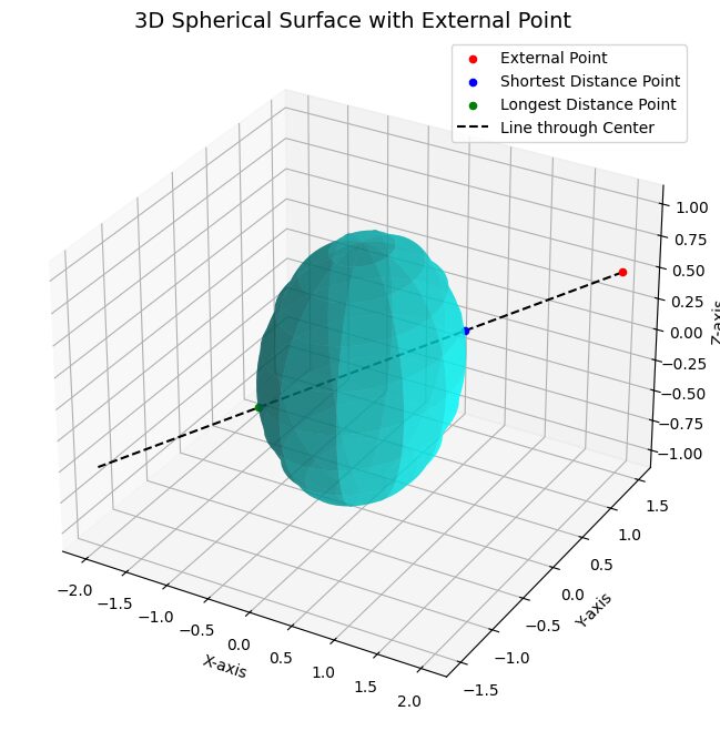
External Point: Red point outside the sphere.
Shortest Distance: Blue point of intersection on the sphere.
Longest Distance: Green point of intersection on the opposite side of the sphere.
Line: Dashed line through the center, connecting the external point and intersection points.
A constraint limits where solutions can occur. For example:
- Circle constraint: [math]x^2 + y^2 = r^2[/math]
- Line constraint: [math]ax + by = c[/math]
Instead of searching everywhere for the best solution, Lagrange multipliers narrow your focus to the constraint’s boundary.
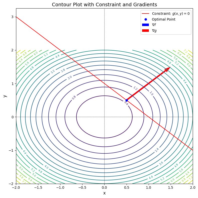
In essence, the gradients of the goal function ([math]\nabla f[/math]) and the constraint ([math]\nabla g[/math]) must align:
[math]\nabla f = \lambda \nabla g[/math].
How Lagrange Multipliers Work
To solve an optimization problem with Lagrange multipliers:
- Define the combined function ([math]\mathcal{L}[/math]):
[math]\mathcal{L}(x, y, \lambda) = f(x, y) + \lambda g(x, y)[/math]. - Take partial derivatives:
[math]\frac{\partial \mathcal{L}}{\partial x}, \frac{\partial \mathcal{L}}{\partial y}, \frac{\partial \mathcal{L}}{\partial \lambda}[/math]. - Solve the system of equations:
[math]\nabla \mathcal{L} = 0[/math], which means:- [math]\frac{\partial \mathcal{L}}{\partial x} = 0[/math]
- [math]\frac{\partial \mathcal{L}}{\partial y} = 0[/math]
- [math]g(x, y) = 0[/math].
Example: To find the maximum value of [math]f(x, y) = x + y[/math] on the circle [math]x^2 + y^2 = 1[/math], you would solve:
[math]\mathcal{L}(x, y, \lambda) = x + y + \lambda (x^2 + y^2 – 1).[/math]
Everyday Examples of Lagrange Multipliers
- Business: Maximize profit ([math]f(x, y)[/math]) while staying within a budget ([math]g(x, y) = 0[/math]).
- Travel: Minimize time ([math]f(x, y)[/math]) while staying on a specific route ([math]g(x, y) = 0[/math]).
For instance, finding the highest point on a hill while restricted to a specific path is a classic problem where Lagrange multipliers shine.
The Geometry of Optimization
The beauty of Lagrange multipliers lies in their geometric interpretation. At the optimal point:
- The goal function’s gradient ([math]\nabla f[/math]) is parallel to the constraint’s gradient ([math]\nabla g[/math]).
- This alignment ensures the constraint is satisfied while optimizing the goal.
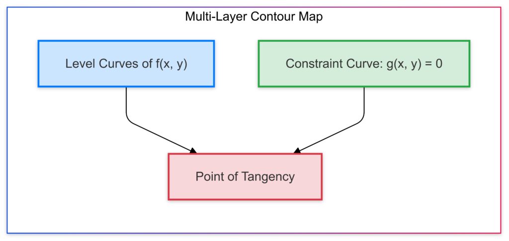
If you visualize a hill (the goal) intersecting a curve (the constraint), the solution is where the curves “touch tangentially.”
Mathematically, this translates to:
[math]\nabla f = \lambda \nabla g[/math]
and the constraint equation: [math]g(x, y) = 0[/math].
Applications of Lagrange Multipliers
Economic Applications
Lagrange multipliers are a cornerstone in economics, especially when optimizing utility or cost.
Utility Maximization
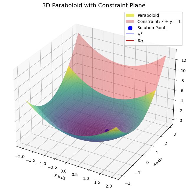
Imagine a consumer trying to maximize their utility [math]U(x, y)[/math] (satisfaction from consuming goods [math](x, y)[/math]) while adhering to a budget constraint:
[math]p_x x + p_y y = M[/math].
To solve this, set up the Lagrangian:
[math]\mathcal{L}(x, y, \lambda) = U(x, y) + \lambda (M – p_x x – p_y y).[/math]
Find partial derivatives:
[math]\frac{\partial \mathcal{L}}{\partial x} = 0, \frac{\partial \mathcal{L}}{\partial y} = 0, \frac{\partial \mathcal{L}}{\partial \lambda} = 0.[/math]
The solution gives the optimal combination of goods [math](x, y)[/math]). Here, [math]\lambda[/math] has an economic interpretation: the marginal utility of money—how much utility increases for every additional dollar spent.
Cost Minimization
For firms, minimizing production costs [math]C(x, y)[/math] under a production requirement constraint [math]g(x, y) = Q[/math] is common. The Lagrange multiplier method provides the optimal input levels for efficiency.
Physics and Engineering Applications
In physics and engineering, constraints often represent physical laws like conservation of energy or material limits.
Example: Minimizing Surface Area
Consider designing a can with fixed volume [math]V = \pi r^2 h[/math]. To minimize surface area:
[math]A = 2\pi r h + 2\pi r^2,[/math]
subject to the volume constraint:
[math]V – \pi r^2 h = 0.[/math]
Define the Lagrangian:
[math]\mathcal{L}(r, h, \lambda) = 2\pi r h + 2\pi r^2 + \lambda (V – \pi r^2 h).[/math]
Take partial derivatives with respect to [math]r, h, and λ[/math], then solve the system:
[math]\frac{\partial \mathcal{L}}{\partial r} = 0, \frac{\partial \mathcal{L}}{\partial h} = 0, \frac{\partial \mathcal{L}}{\partial \lambda} = 0.[/math]
The result determines the optimal ratio of radius to height for the least material use.
Machine Learning and Data Science
Lagrange multipliers play a key role in optimization-heavy fields like machine learning.
Support Vector Machines (SVMs)
SVMs aim to maximize the margin between data classes while adhering to classification constraints. Mathematically:
- Maximize: [math]\frac{1}{2} ||w||^2,[/math]
- Subject to: [math]y_i (w \cdot x_i + b) \geq 1 \ \forall i.[/math]
The Lagrangian incorporates these constraints using multipliers, enabling efficient solutions via dual optimization.
Regularization
In regression, overfitting is controlled by minimizing a loss function [math]L(w)[/math] with a regularization constraint [math]||w|| \leq C[/math]. Lagrange multipliers elegantly handle this trade-off.
Challenges in Higher Dimensions
Visualizing Lagrange multipliers in 3D is relatively straightforward, but what about 4D or higher? While we lose visual intuition, the principles remain: gradients of the goal and constraints must align.
For example, in a multidimensional optimization problem:
- Maximize: [math]f(x_1, x_2, …, x_n),[/math]
- Subject to: [math]g_i(x_1, x_2, …, x_n) = 0 \ \forall i.[/math]
You solve by forming the Lagrangian:
[math]\mathcal{L}(x_1, …, x_n, \lambda_1, …, \lambda_m) = f(x_1, …, x_n) + \sum_{i=1}^m \lambda_i g_i(x_1, …, x_n).[/math]
Numerical solvers like Python’s scipy.optimize simplify these complex problems.

Bridging Theory with Practice
The elegance of Lagrange multipliers lies in how they unify theory and application. They’re used across fields:
- In economics to balance costs and resources.
- In physics to adhere to laws of nature.
- In machine learning to optimize algorithms.
Their ability to handle constraints makes them indispensable in solving real-world problems.
Economic Applications: Utility Maximization
Let’s work through a detailed utility maximization example.
A consumer wants to maximize utility:
[math]U(x, y) = x^{0.5} y^{0.5},[/math]
where xxx and yyy are quantities of two goods, while adhering to the budget constraint:
[math]p_x x + p_y y = M.[/math]
Step 1: Set up the Lagrangian
[math]\mathcal{L}(x, y, \lambda) = x^{0.5} y^{0.5} + \lambda (M – p_x x – p_y y).[/math]
Step 2: Take partial derivatives
Find the first-order conditions by taking partial derivatives:
[math]\frac{\partial \mathcal{L}}{\partial x} = 0, \quad \frac{\partial \mathcal{L}}{\partial y} = 0, \quad \frac{\partial \mathcal{L}}{\partial \lambda} = 0.[/math]
These yield:
[math]\frac{\partial \mathcal{L}}{\partial x} = 0.5 x^{-0.5} y^{0.5} – \lambda p_x = 0,[/math]
[math]\frac{\partial \mathcal{L}}{\partial y} = 0.5 x^{0.5} y^{-0.5} – \lambda p_y = 0,[/math]
[math]\frac{\partial \mathcal{L}}{\partial \lambda} = M – p_x x – p_y y = 0.[/math]
Step 3: Solve the system
From the first two equations:
[math]\frac{0.5 y^{0.5}}{x^{0.5}} = \lambda p_x,[/math]
[math]\frac{0.5 x^{0.5}}{y^{0.5}} = \lambda p_y.[/math]
Equate these to eliminate λ\lambdaλ:
[math]\frac{y}{x} = \frac{p_x}{p_y},[/math]
which simplifies to:
[math]y = \frac{p_x}{p_y} x.[/math]
Substitute into the budget constraint:
[math]p_x x + p_y \left(\frac{p_x}{p_y} x\right) = M,[/math]
[math](p_x + p_x) x = M,[/math]
[math]x = \frac{M}{2p_x}, \quad y = \frac{M}{2p_y}.[/math]
Interpretation
The optimal allocation splits the budget proportionally across goods. The Lagrange multiplier λ\lambdaλ represents how utility changes per additional dollar of budget.
Physics Example: Constrained Particle Motion
Suppose a particle moves on the surface of a sphere:
[math]g(x, y, z) = x^2 + y^2 + z^2 – r^2 = 0.[/math]
You want to minimize the distance to a fixed point :[math](x0,y0,z0)[/math]
[math]f(x, y, z) = (x – x_0)^2 + (y – y_0)^2 + (z – z_0)^2.[/math]
Step 1: Set up the Lagrangian
[math]\mathcal{L}(x, y, z, \lambda) = f(x, y, z) + \lambda g(x, y, z).[/math]
Substituting:
[math]\mathcal{L}(x, y, z, \lambda) = (x – x_0)^2 + (y – y_0)^2 + (z – z_0)^2 + \lambda (x^2 + y^2 + z^2 – r^2).[/math]
Step 2: Take partial derivatives
[math]\frac{\partial \mathcal{L}}{\partial x} = 2(x – x_0) + 2\lambda x = 0,[/math]
[math]\frac{\partial \mathcal{L}}{\partial y} = 2(y – y_0) + 2\lambda y = 0,[/math]
[math]\frac{\partial \mathcal{L}}{\partial z} = 2(z – z_0) + 2\lambda z = 0,[/math]
[math]\frac{\partial \mathcal{L}}{\partial \lambda} = x^2 + y^2 + z^2 – r^2 = 0.[/math]
Step 3: Solve the system
From the first three equations:
[math]x – x_0 = -\lambda x, \quad y – y_0 = -\lambda y, \quad z – z_0 = -\lambda z.[/math]
Rearranging:
[math]x (1 + \lambda) = x_0, \quad y (1 + \lambda) = y_0, \quad z (1 + \lambda) = z_0.[/math]
Solve for λ\lambdaλ using the constraint:
[math]\left(\frac{x_0}{1+\lambda}\right)^2 + \left(\frac{y_0}{1+\lambda}\right)^2 + \left(\frac{z_0}{1+\lambda}\right)^2 = r^2.[/math]
This equation determines [math]λ[/math], and subsequently [math]x, y,[/math] and [math]z [/math].
Interpretation
The solution gives the closest point on the sphere to [math](x0,y0,z0)[/math], adhering to the constraint.
Bridging Insights: Why Use Lagrange Multipliers?
- Efficiency: They elegantly handle constraints without needing to rewrite equations manually.
- Interpretability: The multiplier λ\lambdaλ often has physical or economic meaning, like marginal utility or force balance.
- Generality: Applicable to diverse fields, from geometry to machine learning.
Lagrange multipliers aren’t just theoretical—they’re tools for solving real-world optimization challenges.
Steps to Solve for [math]λ[/math]:
- Factor out [math](1+λ)[/math] in the denominator:
Combine terms under a single denominator:
[math]\frac{x_0^2 + y_0^2 + z_0^2}{(1+\lambda)^2} = r^2.[/math] - Simplify the equation:
Multiply both sides by (1+λ)2(1+\lambda)^2(1+λ)2:
[math]x_0^2 + y_0^2 + z_0^2 = r^2 (1+\lambda)^2.[/math] - Expand the right-hand side:
[math]x_0^2 + y_0^2 + z_0^2 = r^2 (1 + 2\lambda + \lambda^2).[/math] - Rearrange into a quadratic equation:
[math]r^2 \lambda^2 + 2r^2 \lambda + (r^2 – x_0^2 – y_0^2 – z_0^2) = 0.[/math] - Solve for λ\lambdaλ:
Use the quadratic formula:
[math]\lambda = \frac{-2r^2 \pm \sqrt{(2r^2)^2 – 4(r^2)(r^2 – x_0^2 – y_0^2 – z_0^2)}}{2r^2}.[/math] - Simplify further:
[math]\lambda = \frac{-2r^2 \pm \sqrt{4r^4 – 4r^2(r^2 – x_0^2 – y_0^2 – z_0^2)}}{2r^2}.[/math] [math]\lambda = \frac{-2r^2 \pm \sqrt{4r^2(x_0^2 + y_0^2 + z_0^2)}}{2r^2}.[/math] [math]\lambda = \frac{-2r^2 \pm 2r\sqrt{x_0^2 + y_0^2 + z_0^2}}{2r^2}.[/math] [math]\lambda = -1 \pm \frac{\sqrt{x_0^2 + y_0^2 + z_0^2}}{r}.[/math]
Choosing the Correct Root
Since [math](1+λ)[/math] appears in the denominator, we need [math]1+λ>01 [/math]
Thus, choose:
[math]\lambda = -1 + \frac{\sqrt{x_0^2 + y_0^2 + z_0^2}}{r}.[/math]
This value of [math](1+λ)[/math] satisfies the constraint and ensures a valid solution for [math](x,y,z)[/math] .
Final Simplified Solution for [math]λ[/math]
The correct value of [math]λ[/math] is:
[math]\lambda = -1 + \frac{\sqrt{x_0^2 + y_0^2 + z_0^2}}{r}.[/math]
Key Steps Recap:
- Start from the constraint equation:
[math]\frac{x_0^2 + y_0^2 + z_0^2}{(1+\lambda)^2} = r^2.[/math] - Rearrange into a quadratic equation:
[math]r^2 \lambda^2 + 2r^2 \lambda + (r^2 – x_0^2 – y_0^2 – z_0^2) = 0.[/math] - Solve using the quadratic formula, ensuring [math]1+λ>01 [/math]:
[math]\lambda = -1 + \frac{\sqrt{x_0^2 + y_0^2 + z_0^2}}{r}.[/math]
This is the final and valid solution for[math]λ[/math]
Problem Recap
We aim to solve for λ\lambdaλ using the constraint:
[math]\left(\frac{x_0}{1+\lambda}\right)^2 + \left(\frac{y_0}{1+\lambda}\right)^2 + \left(\frac{z_0}{1+\lambda}\right)^2 = r^2.[/math]
This equation ensures the point [math](x,y,z)[/math] lies on the sphere of radius [math]r[/math].
Step-by-Step Solution
- Combine Terms:
Write the left-hand side under a single denominator:
[math]\frac{x_0^2 + y_0^2 + z_0^2}{(1+\lambda)^2} = r^2.[/math] - Eliminate the Denominator:
Multiply through by [math](1+λ)2[/math] to remove the fraction:
[math]x_0^2 + y_0^2 + z_0^2 = r^2 (1+\lambda)^2.[/math] - Expand the Right-Hand Side:
Expand [math](1+λ)2[/math]:
[math]x_0^2 + y_0^2 + z_0^2 = r^2 (1 + 2\lambda + \lambda^2).[/math] - Rearrange into a Quadratic Equation:
Bring all terms to one side to form a quadratic in [math]λ[/math]:
[math]r^2 \lambda^2 + 2r^2 \lambda + (r^2 – x_0^2 – y_0^2 – z_0^2) = 0.[/math] - Solve Using the Quadratic Formula:
The quadratic formula is:
[math]\lambda = \frac{-b \pm \sqrt{b^2 – 4ac}}{2a}.[/math]In this case:- [math]a=r2a = r^2a=r2[/math],[math]b=2r2b = 2r^2b=2r2[/math],[math]c=r2−x02−y02−z02c[/math].
[math]\lambda = \frac{-2r^2 \pm \sqrt{(2r^2)^2 – 4(r^2)(r^2 – x_0^2 – y_0^2 – z_0^2)}}{2r^2}.[/math] - Simplify the Square Root:
Expand the discriminant:
[math]^2 = 4r^4, \quad 4r^2(r^2 – x_0^2 – y_0^2 – z_0^2) = 4r^4 – 4r^2(x_0^2 + y_0^2 + z_0^2).[/math]So, the discriminant becomes:
[math]4r^4 – 4r^4 + 4r^2(x_0^2 + y_0^2 + z_0^2) = 4r^2(x_0^2 + y_0^2 + z_0^2).[/math]The square root is:
[math]\sqrt{4r^2(x_0^2 + y_0^2 + z_0^2)} = 2r\sqrt{x_0^2 + y_0^2 + z_0^2}.[/math] - Simplify the Formula for λ\lambdaλ:
Substitute back into the quadratic formula:
[math]\lambda = \frac{-2r^2 \pm 2r\sqrt{x_0^2 + y_0^2 + z_0^2}}{2r^2}.[/math]Factor out 2r2r2r:
[math]\lambda = -1 \pm \frac{\sqrt{x_0^2 + y_0^2 + z_0^2}}{r}.[/math] - Choose the Correct Root:
To ensure 1+λ>01 + \lambda > 01+λ>0 (since (1+λ)(1+\lambda)(1+λ) is in the denominator of the original equation), select:
[math]\lambda = -1 + \frac{\sqrt{x_0^2 + y_0^2 + z_0^2}}{r}.[/math]
Final Answer
The solution for [math]λ[/math] is:
[math]\lambda = -1 + \frac{\sqrt{x_0^2 + y_0^2 + z_0^2}}{r}.[/math]
This value satisfies the constraint and ensures valid optimization for [math](x,y,z)[/math]
Resources
Books for Deeper Understanding
- “Calculus” by James Stewart
A comprehensive textbook covering multivariable calculus, including Lagrange multipliers. Great for beginners.- Key Feature: Clear examples of constrained optimization in two and three dimensions.
- “Optimization by Vector Space Methods” by David G. Luenberger
A deeper dive into optimization theory, ideal for those with a strong math background.- Key Feature: Covers Lagrange multipliers and their extensions like KKT conditions.
- “Convex Optimization” by Stephen Boyd and Lieven Vandenberghe
A modern classic, covering optimization methods widely used in engineering and data science.- Key Feature: Connects Lagrange multipliers with real-world applications like machine learning.
Online Courses and Tutorials
- Khan Academy (Multivariable Calculus)
- Offers a friendly introduction to Lagrange multipliers with interactive visuals.
- Link: Khan Academy
- MIT OpenCourseWare: Multivariable Calculus
- Free lecture videos and notes from MIT professors. Perfect for building foundational understanding.
- Link: MIT OCW
- Brilliant.org – Multivariable Calculus Pathway
- Interactive lessons and problem-solving activities on Lagrange multipliers and gradients.
- Link: Brilliant.org
Tools for Visualization and Practice
- Desmos (2D Graphing Calculator)
- Plot constraints and contours to visualize Lagrange multiplier solutions interactively.
- Link: Desmos
- GeoGebra
- Excellent for 3D visualization of constraint surfaces and gradient alignment.
- Link: GeoGebra
- Python Libraries: SymPy and Matplotlib
- Use SymPy for symbolic math and Matplotlib for contour visualizations. Example:
import numpy as np import matplotlib.pyplot as plt x = np.linspace(-2, 2, 400) y = np.linspace(-2, 2, 400) X, Y = np.meshgrid(x, y) Z = X + Y # Example function constraint = X**2 + Y**2 - 1 plt.contour(X, Y, Z, levels=20, cmap='viridis') plt.contour(X, Y, constraint, levels=[0], colors='red') plt.title("Contours and Constraint") plt.show()

Research Papers and Advanced Resources
- “On the Multipliers in Optimization” by Hestenes
A classic research paper on the theoretical basis of Lagrange multipliers. - “Mathematics of Machine Learning” (Stanford CS229 Notes)
- Explains how Lagrange multipliers apply to optimization in machine learning.
- Link: Stanford CS229
Community Resources
- Stack Exchange: Mathematics
- Post specific questions and get answers from experts.
- Link: Mathematics Stack Exchange
- Reddit: Learn Math
- Join discussions and ask questions in a beginner-friendly space.
- Link: r/learnmath