
Simulated annealing (SA) is a powerful optimization algorithm inspired by the annealing process in metallurgy. To unlock its potential, tuning parameters properly is key. Let’s dive into the best practices and strategies for parameter optimization in SA.
Understanding the Core Parameters of Simulated Annealing
What Makes Simulated Annealing Tick?
At its core, SA relies on temperature and cooling schedules. These control the exploration of the solution space.
- Initial temperature: Sets how far the algorithm can explore. Too high, and you’ll waste time. Too low, and it’s narrow-minded.
- Cooling rate: Governs how quickly temperature drops. Think of it as balancing exploration with exploitation.
- Stopping criteria: Decides when the algorithm halts—key for efficiency.
The interplay between these parameters defines the algorithm’s success. Missteps can lead to poor convergence or wasted resources.
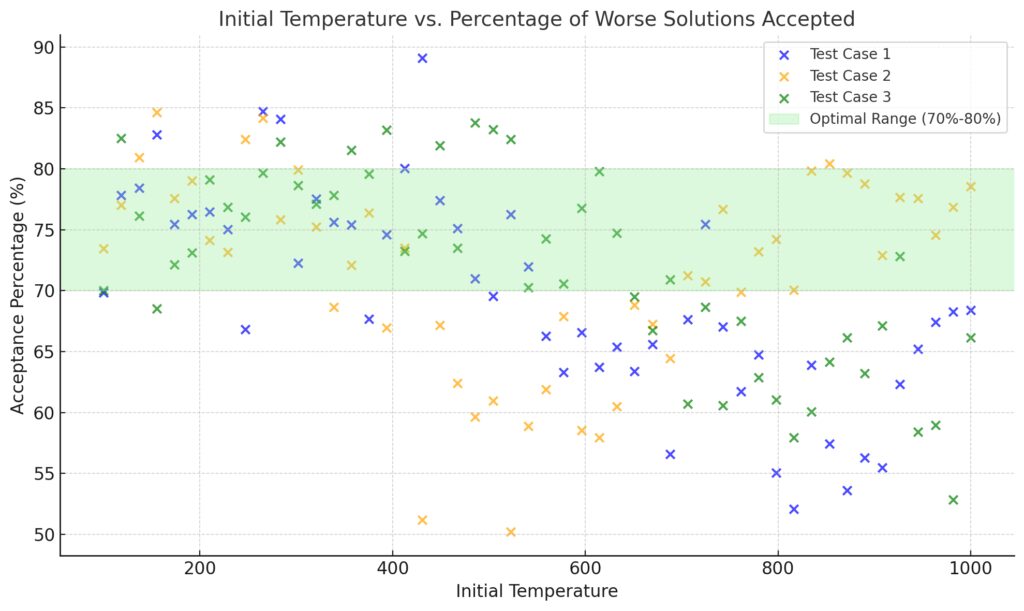
Optimal Range: The shaded green region indicates the optimal acceptance percentage (70%-80%), where the system balances exploration and convergence effectively.
Why Tuning Parameters Is Crucial
If parameters are poorly configured, the algorithm risks:
- Getting stuck in local optima.
- Missing the global optimum altogether.
- Running inefficiently, wasting computational resources.
A good parameter setup ensures both a thorough exploration of the solution space and timely convergence.
Mastering the Cooling Schedule for Balanced Convergence
The Role of the Cooling Rate
The cooling rate determines how the temperature decreases over time. Popular cooling schedules include:
- Linear cooling: Simple but may converge too fast.
- Exponential cooling: Provides a steady decrease, often preferred for fine-tuning.
- Adaptive cooling: Adjusts based on feedback, balancing exploration and convergence dynamically.
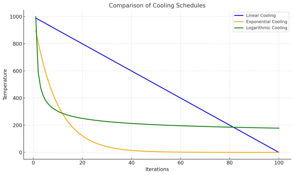
Linear Cooling: Temperature decreases linearly with each iteration.
Exponential Cooling: Temperature decreases exponentially, showcasing rapid cooling in initial iterations.
Logarithmic Cooling: Temperature decreases slowly, maintaining a higher temperature for longer.
Tips for Effective Cooling
- Slower cooling promotes thorough exploration but takes more time.
- Faster cooling speeds up the process but may miss the global optimum.
Test various schedules to find the sweet spot for your problem.
Examples of Cooling Functions
Mastering the Cooling Schedule for Balanced Convergence
The Role of the Cooling Rate
The cooling rate determines how the temperature decreases over time. Popular cooling schedules include:
- Linear cooling: Simple but may converge too fast.
- Exponential cooling: Provides a steady decrease, often preferred for fine-tuning.
- Adaptive cooling: Adjusts based on feedback, balancing exploration and convergence dynamically.
Tips for Effective Cooling
- Slower cooling promotes thorough exploration but takes more time.
- Faster cooling speeds up the process but may miss the global optimum.
Test various schedules to find the sweet spot for your problem.
Examples of Cooling Functions
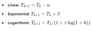
Each method suits different optimization landscapes.
Defining the Neighborhood: Local Exploration Strategies
Choosing a Neighborhood Function
The neighborhood function defines how candidate solutions are generated. This choice directly impacts performance.
- Small perturbations: Ideal for fine-tuning but may slow down progress.
- Larger jumps: Better for initial exploration, but they risk overshooting optimal regions.
Match the function to your problem type. For example:
- Use bit-flipping for binary optimization problems.
- Try Gaussian perturbations for continuous variables.
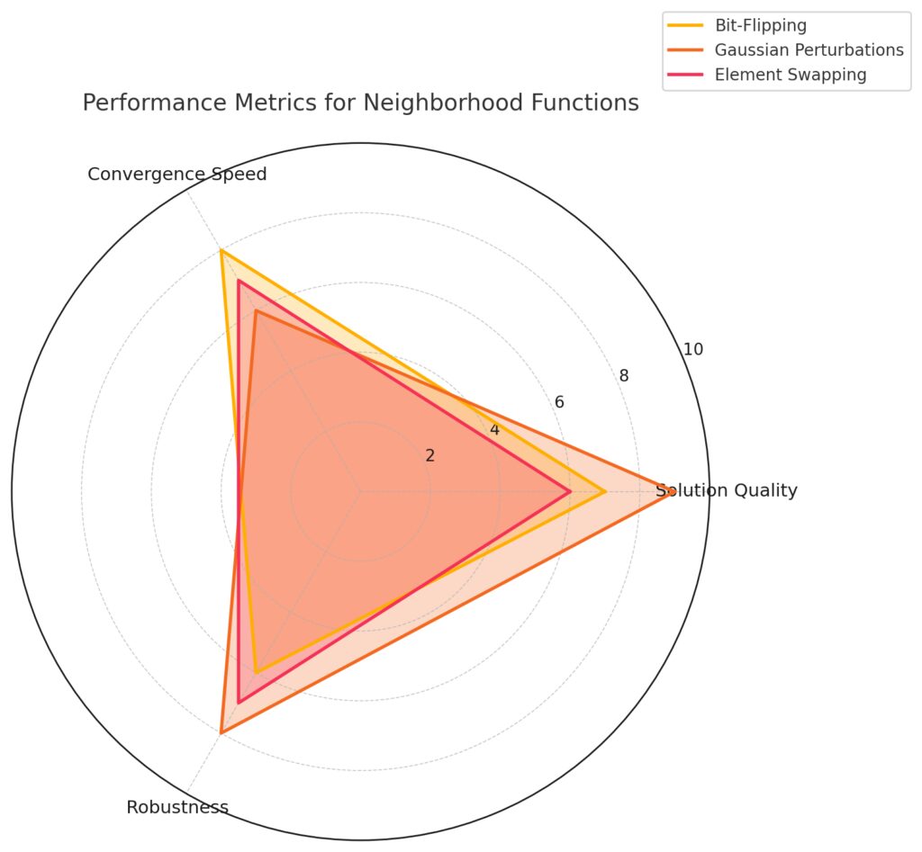
Convergence Speed: Evaluates how quickly the method converges to a solution.
Robustness: Assesses consistency across different problem instances.
Key Insights:
Bit-Flipping: High convergence speed and good solution quality but slightly lower robustness.
Gaussian Perturbations: Excels in solution quality and robustness but has a lower convergence speed.
Element Swapping: Balanced across all metrics, with no extreme highs or lows.
Balancing Local vs. Global Search
The neighborhood size should shrink as the temperature decreases. This helps the algorithm focus on the best regions near the end.
Stopping Criteria: Knowing When to Call It Quits
Common Stopping Rules
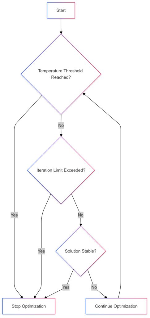
Stopping criteria prevent wasted computation. Popular approaches include:
- Temperature threshold: Stop when the temperature drops below a minimum.
- Iteration limit: Useful for time-sensitive applications.
- Solution stability: Stop if no improvement occurs for several iterations.
Dynamic Stopping Methods
Advanced techniques analyze improvement trends to predict diminishing returns. Use them to optimize runtime without sacrificing solution quality.
Advanced Techniques for Tuning Simulated Annealing Parameters
Mastering basic parameters is essential, but advanced techniques take your simulated annealing (SA) game to the next level. Let’s explore methods for dynamic tuning, adaptive strategies, and leveraging tools to optimize parameter selection.
Adaptive Simulated Annealing: Dynamic Adjustment in Action
What Is Adaptive SA?
Unlike standard SA, where parameters remain fixed, adaptive simulated annealing adjusts parameters on the fly. It responds to the problem’s landscape and performance metrics, ensuring optimal behavior.
How It Works
- Temperature adjustments: Modify the cooling rate or initial temperature based on solution quality.
- Dynamic neighborhood sizes: Shrink or expand neighborhood size depending on the stage of optimization.
- Feedback loops: Use historical data to refine acceptance probabilities and stopping conditions.
For example, if improvement stalls, a temporary increase in temperature can jumpstart exploration.
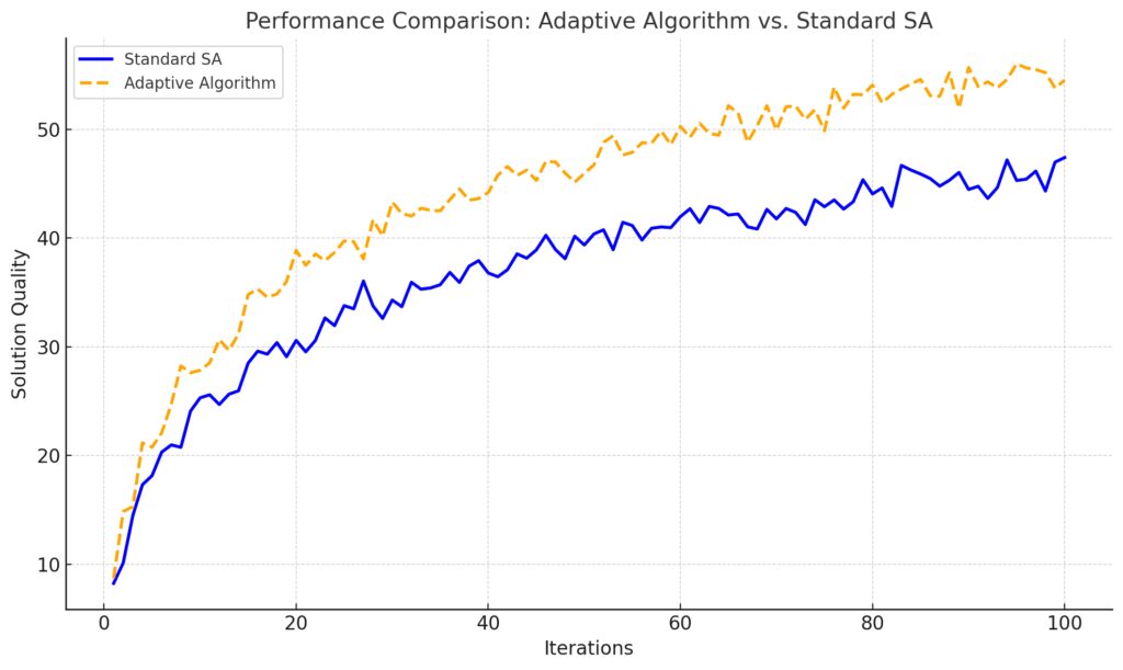
Standard SA: Progresses steadily, showing consistent improvement in solution quality.
Adaptive Algorithm: Outperforms standard SA, achieving higher solution quality at most iterations, indicating its efficiency in adaptation.
Benefits of Adaptivity
- Improved convergence to global optima.
- Greater efficiency, saving time and computational resources.
- Robustness across diverse problem domains.
Parameter Sweeps: Testing for the Best Settings
Conducting Systematic Experiments
Parameter sweeps involve testing a range of values for one or more parameters to find the ideal combination. For example:
- Vary the cooling rate from 0.85 to 0.99 in increments of 0.02.
- Experiment with neighborhood functions and measure solution quality.
Use grids or random sampling to ensure coverage across the parameter space.
Evaluating Performance
Key metrics for assessing SA performance include:
- Convergence time: How quickly does the algorithm find good solutions?
- Solution quality: Compare against known benchmarks or other algorithms.
- Stability: Ensure performance is consistent across runs.
Statistical tools like ANOVA or response surface methodology can pinpoint the best settings.
Hybrid Approaches: Combining SA with Other Algorithms
Why Combine Simulated Annealing?
While SA excels at escaping local optima, it can be slow for fine-tuning. Hybrid algorithms combine SA with other optimization techniques to overcome these limitations.
Examples of Hybrid Approaches
- SA + Genetic Algorithms (GA): Use GA for global search and SA for local refinement.
- SA + Tabu Search: Avoid revisiting solutions while maintaining randomness in SA.
- SA + Gradient Descent: Apply gradient-based methods when SA converges near the optimum.
Benefits of Hybrids
- Faster convergence.
- Enhanced accuracy for complex or high-dimensional problems.
- Flexibility for multi-objective optimization.
Tools and Libraries for Simulated Annealing Optimization
Popular SA Libraries
Several libraries make implementing and tuning SA easier:
- SciPy: Offers a robust
dual_annealingfunction for global optimization in Python. - Simulated Annealing for Matlab: User-friendly for testing and visualization.
- HeuristicLab: A flexible framework for heuristic and evolutionary algorithms.
Automation Tools
- Hyperopt: Ideal for tuning hyperparameters of SA algorithms.
- Optuna: Automates parameter optimization with state-of-the-art algorithms.
Practical Tips for Effective Parameter Tuning
1. Start with Defaults, Then Refine
Many libraries provide reasonable defaults. Use these as a baseline and refine parameters iteratively.
2. Analyze the Problem Domain
Tailor parameters to your specific problem. For instance:
- Use slower cooling for rugged landscapes.
- Opt for higher initial temperatures if local optima are common.
3. Monitor and Log Results
Track metrics like solution quality, runtime, and iteration count. Logs provide insights for future tuning and comparisons.
4. Avoid Overfitting Parameters
Don’t design parameters to work perfectly for one test case at the expense of general performance.
Conclusion: Mastering Simulated Annealing
Tuning parameters in simulated annealing is as much art as science. By understanding the basics, leveraging adaptive strategies, and using advanced tools, you can maximize performance for any optimization problem. Remember: experimentation and analysis are your best guides. With careful tuning, SA can solve even the toughest challenges.
FAQs
What is the best cooling schedule to use in simulated annealing?
The best cooling schedule depends on the problem.
- Exponential cooling is commonly effective for smooth optimization problems. Example: Finding optimal routes in logistics systems.
- Linear cooling works well for time-sensitive tasks but risks premature convergence. Example: Quick approximations in scheduling.
- Adaptive cooling dynamically adjusts based on performance, excelling in diverse or rugged solution spaces. Example: Circuit design optimization.
Testing different schedules on small datasets or subsets of the problem helps determine the ideal approach.
How do I decide on the initial temperature?
The initial temperature should allow the algorithm to explore the solution space broadly without overdoing it.
A useful heuristic is to set the temperature so that around 80% of worse solutions are accepted initially. For instance:
- If optimizing manufacturing processes, set a high initial temperature to explore different layouts.
- For refining machine learning models, a moderate temperature often suffices.
Experimentation with empirical acceptance rates will guide fine-tuning.
How can I avoid the algorithm getting stuck in local optima?
Three strategies help mitigate this risk:
- Set a higher initial temperature to encourage wide exploration.
Example: In job shop scheduling, a higher temperature can explore various task sequences before narrowing in. - Adjust the neighborhood size dynamically, shrinking it as the temperature decreases.
Example: Begin with significant perturbations in investment portfolio optimization, then refine allocations. - Introduce randomness periodically by temporarily increasing the temperature.
Example: When designing games, randomness might help overcome design bottlenecks.
What neighborhood functions should I use?
Neighborhood functions depend on the problem’s structure.
- For binary problems, such as feature selection, bit-flipping works well. Example: Turning features on/off in a machine learning model.
- For continuous variables, Gaussian perturbations or random walks are ideal. Example: Adjusting parameters in a chemical reaction model.
- For permutation problems, like the traveling salesman problem, swapping elements is effective. Example: Exchanging city order in a route.
The chosen function should align with the problem’s domain to balance exploration and precision.
When should I stop the algorithm?
Stopping criteria should balance thorough exploration with computational efficiency.
- Fixed temperature threshold: Stop when temperature drops below a set value. Example: When optimizing ad placements, halt when no further meaningful gains occur.
- Iteration limit: Useful for time-sensitive problems. Example: Budget analysis with strict deadlines.
- Solution stability: Stop when no improvements occur for a predefined number of iterations. Example: Refining manufacturing layouts where the best configurations stabilize quickly.
Dynamic stopping criteria, like monitoring diminishing returns, can enhance efficiency.
How can I tune the cooling rate effectively?
Tuning the cooling rate requires balancing exploration and convergence.
- A slower cooling rate (e.g., 0.99) allows thorough exploration and works well for highly complex landscapes.
Example: Optimizing neural network hyperparameters, where solutions may lie in narrow, hard-to-reach regions. - A faster cooling rate (e.g., 0.85) speeds up the process but risks missing the global optimum.
Example: Quick adjustments in workforce scheduling to meet tight deadlines.
Start with a moderate rate like 0.95 and adjust based on observed performance.
What is the role of randomness in simulated annealing?
Randomness prevents the algorithm from getting stuck in suboptimal solutions.
- Random solution generation enables jumps to unexplored areas of the solution space. Example: In warehouse design, randomness might generate layouts that wouldn’t be considered otherwise.
- Acceptance of worse solutions allows escape from local optima. Example: Accepting a higher-cost route in logistics temporarily might reveal better alternatives later.
Carefully control the randomness by adjusting the temperature and acceptance probability.
How do I benchmark the performance of my SA implementation?
Benchmarking involves comparing SA’s performance against known results or alternative methods.
- Use test cases with known optimal solutions. Example: Solving a standard traveling salesman problem instance for validation.
- Compare solution quality and convergence speed with other algorithms like genetic algorithms or gradient descent. Example: Use both methods for supply chain optimization and evaluate which performs better.
- Track metrics such as average improvement per iteration and stability of results across runs.
Consistency across multiple problem instances signals effective parameter tuning.
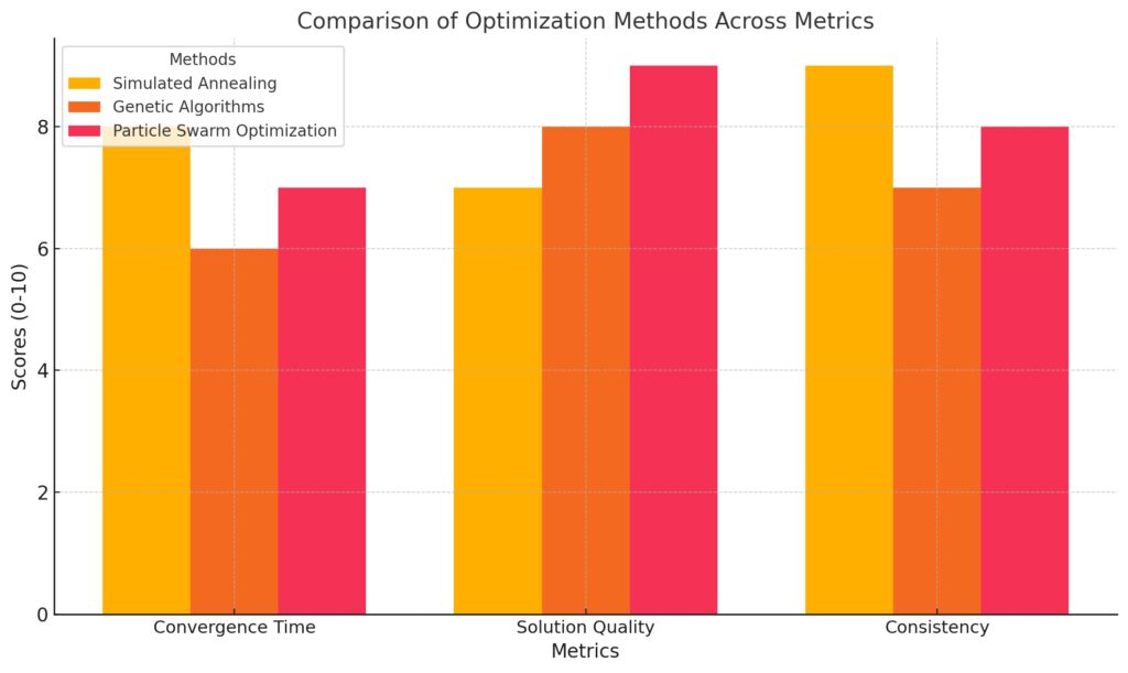
Solution Quality: Particle Swarm Optimization leads, with Genetic Algorithms closely behind.
Consistency: Simulated Annealing is the most consistent, reflecting its stability in finding reliable solutions.
What problems are unsuitable for simulated annealing?
SA isn’t ideal for problems where:
- Precise solutions are required quickly. Example: Real-time navigation in fast-changing environments, where SA’s exploratory nature might lag.
- Gradient-based methods work better. Example: Deep learning optimization, where gradients can be directly calculated.
- Deterministic paths are more effective. Example: Solving Sudoku puzzles, which require logic-based solutions rather than randomness.
However, for problems with vast search spaces and no clear gradients, SA shines.
Can simulated annealing handle multi-objective optimization?
Yes, SA can handle multiple objectives with some modifications.
- Use weighted sums to combine objectives into a single value. Example: Balancing cost and delivery time in supply chain optimization.
- Try Pareto-based approaches, where multiple solutions are maintained simultaneously. Example: In designing eco-friendly buildings, explore trade-offs between energy efficiency and construction cost.
Specialized versions, like multi-objective simulated annealing (MOSA), are tailored for such problems.
How do I choose between standard and adaptive simulated annealing?
The choice depends on your problem and resources.
- Standard SA is suitable for problems where the landscape is predictable and computational resources are limited.
Example: Optimizing machine layouts in manufacturing, where the constraints are well-understood. - Adaptive SA shines in dynamic or unknown problem spaces.
Example: Optimizing financial portfolios in volatile markets, where adaptability can handle sudden changes.
If you’re unsure, start with standard SA and switch to adaptive methods if performance stalls.
What are some common pitfalls in tuning simulated annealing?
Avoid these mistakes to maximize SA’s effectiveness:
- Setting a cooling rate too high or too low.
Too high causes premature convergence, while too low wastes computational resources. Example: Overcooling in a network optimization problem may leave gaps in solutions. - Skipping experimentation with initial parameters.
Default parameters might not suit your specific problem. Example: A low initial temperature in feature selection may ignore better subsets. - Ignoring problem-specific constraints.
Customizing neighborhood functions and acceptance criteria for the task is crucial. Example: Permutation constraints in vehicle routing must be respected to avoid infeasible routes.
Iterative testing and problem-specific customization are key to avoiding these issues.
Can simulated annealing be parallelized?
Yes, though SA is inherently sequential, certain aspects can benefit from parallelism:
- Parallel evaluations of neighborhoods: Test multiple candidate solutions simultaneously. Example: In optimizing server configurations, evaluate parallel server setups.
- Independent runs: Run multiple instances with different initial parameters or seeds. Example: Multi-start SA in logistics optimizes routes faster by aggregating results.
- Hybrid parallelism: Combine SA with parallel algorithms, like genetic algorithms, for global and local optimization.
Frameworks like OpenMP or GPU-based tools can help implement parallelization.
How do I handle constraints in simulated annealing?
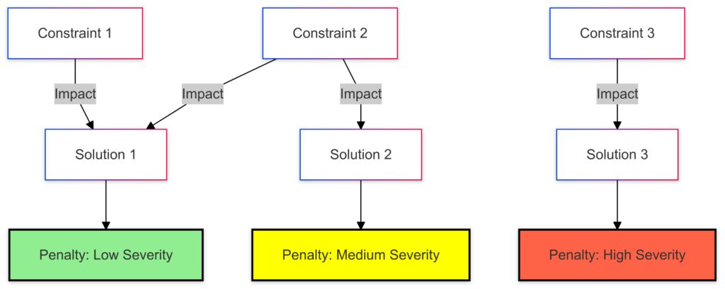
Constraints can be managed through creative modifications to the algorithm:
- Penalty functions: Add penalties to the objective function for violating constraints. Example: Penalize exceeding weight limits in knapsack problems.
- Repair functions: Adjust solutions to meet constraints after perturbations. Example: Correcting a routing sequence in a traveling salesman problem to maintain feasibility.
- Hard constraints: Reject infeasible solutions outright. Example: In manufacturing schedules, reject solutions that don’t meet delivery deadlines.
The choice depends on the complexity and strictness of your constraints.
Are there alternatives to simulated annealing for large problems?
While SA is powerful, alternatives might work better for very large or specific problems:
- Genetic algorithms (GA): Better for multi-objective or highly combinatorial problems. Example: Evolving product designs.
- Particle swarm optimization (PSO): Efficient for continuous optimization tasks. Example: Tuning machine learning hyperparameters.
- Tabu search: Great for discrete problems with local search focus. Example: Staff scheduling.
- Ant colony optimization: Effective for routing and pathfinding. Example: Delivery routing in urban areas.
These methods often complement SA in hybrid approaches for tackling complex problems.
Resources
Open-Source Libraries
- Python’s SciPy Library
Thedual_annealingfunction in SciPy provides a robust implementation of simulated annealing for global optimization problems. - Simulated Annealing for MATLAB
MATLAB’s optimization toolbox includes SA implementations with easy customization for engineering and scientific applications. - Simanneal (Python)
A lightweight Python library for implementing simulated annealing with adjustable parameters. Check it out on GitHub.
Academic and Practical Case Studies
- IEEE Xplore Digital Library
Explore cutting-edge research papers detailing the latest advancements and applications of simulated annealing. Example topics include scheduling, logistics, and AI optimization. - ResearchGate
Access user-shared studies and implementations, such as applications of SA in real-world scenarios like energy optimization and supply chain design. - Kaggle Datasets and Notebooks
Search for practical implementations of simulated annealing applied to competitive problems, such as route optimization or hyperparameter tuning.
Tools for Experimentation
- Optuna
A hyperparameter optimization framework that automates parameter tuning for SA and other algorithms. Learn more here. - Hyperopt
An open-source library for optimizing the performance of simulated annealing configurations through Bayesian search. - HEALPy (Heuristic Algorithms Library in Python)
Provides implementations of heuristic algorithms, including simulated annealing, with customizable cooling schedules and neighborhood functions.